Fun with DSP
I've had some dsPIC33FJ128GP802s Sitting around for many years. I always wanted to use them for DSP applications, in particular audio, but never got around to using them. I ended up using them for a job so finally got a chance to use them.
Out of Microcontrollers I prefer the PIC chips from Microchip. They aren't perfect and they do have bugs in them, but, the documentation is very extensive and you have total control with them. Maybe it's just because I've had more experience with them but I find the Arduino way of doing things very limiting. Quite often I am designing some piece of hardware that needs say to use the least amount of energy possible. With pic chips I find this quite easy as at any one time I can figure out exactly what they are doing and I can switch off modules inside them to reduce power when appropriate. I find Arduino okay for throwing together quick sketches but I'm never quite sure what's going on and that lack of understanding bothers me. The infamous ARM chips these days are very popular and find their ways into cell phones and pretty much everything. However, I don't have any experience using them at a low level so have no idea what goes on inside them. I only find micro processors fun when I have total control over them, can go to an arbitrarily low level of programming, and the documentation is good enough that it can help me been them to my will.
After using the dsPIC33FJ128GP802 chip a bit I must admit it's a nice chip! It has some very cool features that you don't realize are so cool until you start using it. It's a fixed point 16-bit microcontroller that runs up to 80MHz and its speed is about 40MIPS. So looking on the MIPS wiki page that looks comparable to a 486 or an ARM7 speed wise. So that doesn't sound that impressive. However, the architecture is interesting, it has dual port RAM, two address buses, a DMA Controller that doesn't steal CPU cycles and is totally transparent, hardware circular buffers, zero overhead loops, the wonderful MAC command, most commands a one or two cycles, and a whole lot of other neat commands and things. Here are the specs The Microchip webpage gives...
Operating Range
- Up to 40 MIPS operation (at 3.0-3.6V)
- 3.0V to 3.6V, -40ºC to +125ºC, DC to 40 MIPS
High-Performance dsPIC33FJ core- Modified Harvard architecture
- C compiler optimized instruction set
- 24-bit wide instructions, 16-bit wide data path
- Linear program memory addressing up to 4M instruction words
- Linear data memory addressing up to 64 Kbytes
- Two 40-bit accumulators with rounding and saturation options
- Indirect, Modulo and Bit-reversed addressing modes
- 16 x 16 fractional/integer multiply operations
- 32/16 and 16/16 divide operations
- Single-cycle multiply and accumulate (MAC) with accumulator write back and dual data fetch
- Single-cycle MUL plus hardware divide
- Up to ±16-bit shifts for up to 40-bit data
- On-chip Flash and SRAM
Direct Memory Access (DMA)
- 8-channel hardare DMA
- Up to 2 Kbytes dual ported DMA buffer area (DMA RAM) to store data transferred via DMA
- Most peripherals support DMA
Timers/Capture/Compare/PWM
- Up to five 16-bit and up to two 32-bit Timers/Counters
- One timer runs as a Real-Time Clock with an external 32.768 kHz oscillator
- Input Capture (up to four channels) with Capture on up, down or both edges
- 16-bit capture input functions
- 4-deep FIFO on each capture
- Output Compare (up to four channels) with Single or Dual 16-bit Compare mode and * 16-bit Glitchless PWM mode
- Hardware Real-Time Clock/Calendar (RTCC)
Interrupt Controller
- 5-cycle latency
- 118 interrupt vectors
- Up to 49 available interrupt sources
- Up to three external interrups
- Seven programmable priority levels
- Five processor exceptions
Digital I/O
- Peripheral pin Select functionality
- Up to 35 programmable digital I/O pins
- Wake-up/Interrupt-on-Change for up to 21 pins
- Output pins can drive from 3.0V to 3.6V
- Up to 5V output with open drain configuration
- All digital input pins are 5V tolerant
- 4 mA sink on all I/O pins
System Management
- Flexible clock options: External, crystal, resonator and internal RC
- Fully integrated Phase-Locked Loop (PLL)
- Extremely low jitter PLL
- Power-up Timer
- Oscillator Start-up Timer/Stabilizer
- Watchdog Timer with its own RC oscillator
- Fail-Safe Clock Monitor
- Reset by multiple sources
Power Management
- On-chip 2.5V voltage regulator
- Switch between clock sources in real time
- Idle, Sleep, and Doze modes with fast wake-up
Analog-to-Digital Converters (ADCs)
- 10-bit, 11 Msps or 12-bit, 500 Ksps conversion
- Two and four simultaneous samples (10-bit ADC)
- Up to 13 input channels with auto-scanning
- Conversion start can be manual or synchronized with one of four trigger sources
- Conversion possible in Sleep mode
- ±2 LSb max integral nonlinearity
- ±1 LSb max differential nonlinearity
Other Analog Peripherals
- Two analog comparators with programmable input/output configuration
- 4-bit DAC with two ranges for analog comparators
- 16-bit dual channel 100 Ksps audio DAC
Data Converter Interface (DCI) module
- Codec interface
- Supports I2S and AC.97 protocols
- Up to 16-bit data words, up to 16 words per frame
- 4-word deep TX and RX buffers
Communication Modules
- 4-wire SPI (up to two modules) with I/O interface to simple codecs
- I2C™ with Full Multi-Master Slave mode support, slave address masking, 7-bit and 10-bit addressing, integrated signal conditioning and bus collision detection
- UART (up to two modules) with LIN bus support, IrDA® and hardware flow control with CTS and RTS
- Enhanced CAN (ECAN) module (1 Mbaud) with 2.0B support
- Parallel Master Slave Port (PMP/EPSP)
- Programmable Cyclic Redundancy Check (CRC)
Debugger Development Support
- In-circuit and in-application programming
- Two program breakpoints
- Trace and run-time watch
I think that's enough to make anyone's eyes glaze over.
Putting some hardware together
Anyway let's put together some basic hardware that we can use for audio processing DSP tasks. The chips have an ADC and a DAC on them so we can send audio to the chip using the ADC and obtain audio from the chip using the DAC. This allows us to put code on the chip to perform DSP on the input and output audio. My chips came in the DIP format but you can also get them in SMD formats. The advantage of the DIP format is prototyping is easy and can be done on veroboard or breadboard.

dsPIC33FJ128GP802 pinout
I was slack with the hardware and just threw together whatever bits I had lying around so hence some strange values of components. Also, I didn't bother to put a buffer on the input of the ADC. The two resistors on pin two are so small that anything below 1 kHz gets attenuated a lot. Let's call this hardware version one and learn from it.

Hardware version 1 schematic
J1 is the PIC header for the Microchip programmer. TXD and RXD are for the serial to USB converter. The power lines are VDD and GND and also go to the USB converter, this is where the dsPIC chip gets its power from.

Hardware version 1 in real life
Software
Now we have to put some software on the chip. I almost always use Qt Creator as an IDE to write C/C++ programs. I think it's a great IDE and has great code completion.
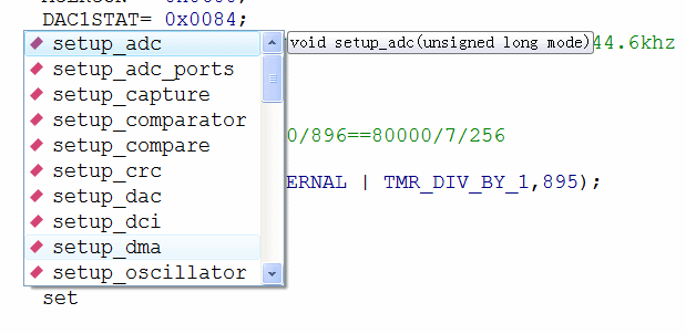
Qt Creator with code completion pop-up window
So I'm going to use Qt Creator to write code for the dsPic chip. For the compiler I usually use a CCS C Compiler, the compiler is a little bit buggy but it's easy to use. For burning the software to the dsPic chip I use a PICKit 3 and an old version of MPLAB (v8.92) as I don't like the new version of MPLAB. I also use MPLAB for debugging.
I use the CCS C Compiler somewhat like a tutor. It has easy to use commands like setup_dma(0, DMA_IN_ADC1, DMA_WORD);. They may not be very customizable commands but you can look at the assembly language that they produce and work out what they are doing with the help of the microchip documentation. At that point you can do little tweaks to them, remove the C command and replace it with assembly language. I find it is easier doing it this way than trying to understand everything about the module inside the dsPic. The following shows an example of me having a look to see what the two commands setup_dma and dma_start do...
....................     setup_dma(0, DMA_IN_ADC1, DMA_WORD);
03F14:  CLR.B   381		CHEN=0,SIZE=0,DIR=0,HALF=0,NULW=0 (DMA0CON)
03F16:  MOV.B   #D,W0L		IRQSEL=13 (DMA0REQ)
03F18:  MOV.B   W0L,382
03F1A:  MOV     #300,W4		PAD=&ADC1BUF0 (DMA0PAD)
03F1C:  MOV     W4,388
....................     dma_start(0, DMA_CONTINOUS|DMA_PING_PONG, &DMA_ADC_Buffer[0],&DMA_ADC_Buffer[DMA_BUFFER_SIZE],DMA_BUFFER_SIZE-1 );
03F1E:  BCLR.B  381.7		CHEN=0 (DMA0CON)
03F20:  MOV.B   #2,W0L		MODE=2,AMODE=0 (DMA0CON)
03F22:  MOV.B   W0L,380
03F24:  MOV     #4000,W4	STA=0x4000 (DMA0STA)
03F26:  MOV     W4,384
03F28:  MOV     #4014,W4	STB=0x4014 (DMA0STB)
03F2A:  MOV     W4,386
03F2C:  MOV     #9,W4		CNT=9 (DMA0CNT)
03F2E:  MOV     W4,38A
03F30:  BSET.B  381.7		CHEN=1 (DMA0CON)
For the dsPic I also use this inspecting the assembly language to work around compiler bugs and to significantly speed up code execution. The following is supposed to remove the DC bias from a 16 bit signed integer. It doesn't work. The compiler is using a logical shift right (LSR) rather than an arithmetic shift right (ASR) even though dc_bias is a 32 bit signed integer. Wikipedia says...
"Most C and C++ implementations, and Go, choose which right shift to perform depending on the type of integer being shifted: signed integers are shifted using the arithmetic shift, and unsigned integers are shifted using the logical shift."
So this is one that doesn't.
....................                 //correct for dc bias
....................                 val-=(dc_bias>>17);
03F56:  MOV     #11,W4
03F58:  MOV     197A,W5
03F5A:  MOV     197C,W6
03F5C:  INC     W4,W4
03F5E:  DEC     W4,W4
03F60:  BRA     Z,3F68
03F62:  LSR     W6,W6
03F64:  RRC     W5,W5
03F66:  BRA     3F5E
03F68:  MOV     1FFE,W0
03F6A:  CLR     W1
03F6C:  BTSC    W0.F
03F6E:  SETM    W1
03F70:  SUB     W0,W5,W0
03F72:  SUBB    W1,W6,W1
03F74:  MOV     W0,1FFE
Looking through the Microchip programming documentation the command we wish to use is called ASR and only requires three instructions rather than the 16 we had before...
....................                 //correct for dc bias (val-=(dc_bias>>17); with arithmetic
....................                 #asm
....................                     MOV dc_bias+2,W0;
03F50:  MOV     197C,W0
....................                     ASR W0,#1,W0;
03F52:  ASR     W0,#1,W0
....................                     SUB val;
03F54:  SUB     1FFC
....................                 #endasm
This means if the micro processor was running at 100% doing nothing but the original incorrect code, then, the new code would use less than 20%; that's a significant savings. This kind of thinking is important with DSP as it's easy to use 100% of CPU even on a powerful modern computer if you're not careful.
With that in mind we have to create a way where we are given two buffers, one that is empty that can be filled with data that will go to the DAC, and another that is full and we can empty that comes from the ADC. We have to receive both these buffers at the same time, we need time to process these two buffers, the DAC and the ADC must run at exactly the same speed and almost in the same phase with one another, and the buffers have to be the same size. In addition, we would like it if the CPU did not have to do any work to obtain these two buffers so as to have more time to process the buffers. Fortunately, in the DSPic there are enough modules to allows to do this.
I find both the ADC and the DAC in the DSPic rather strange. They don't entirely match each other...
The ADC requires that you sample the input voltage, wait a while, disconnect the input voltage, start a conversion of the voltage that is on the capacitor, wait for that conversion to finish. On the face of it the doesn't look any way of automating this procedure. However, it is possible to automatically sample after a conversion has finished. That still leaves how do you get it to start a conversion. Well, fortunately timer three can be set up such that when it times out it will start a conversion. So that will cause the ADC to repeatedly update a memory location with the value that represents the voltage on the ADC input. It's just one memory location and has no buffering. Also the ADC is only 12 bits.

ADC operation
On the other hand there are two DACs that have 16 bits, some sort of oversampling that I don't understand, have limited buffering, automatic sampling/conversion, and have differential outputs. Clearly the DAC is set up for audio applications while the ADC not so much. The DAC's clock source comes from higher up in the multiplications and divisions of the primary oscillator that happen in the dsPIC chip. This can make it difficult to get the frequency of the automatic sampling/conversion right, but once you've done that the rest of the DAC is pretty easy to use. To supply with data you can push a few samples into a register and the DAC will move them into the analog world; still it's not much of a buffer.

DAC operation
So, to make sure that they're running at exactly the same speed with respect to one another they need to be run from the same oscillator source which can be done and is the internal source. Timer three can be set to timeout with the exact same speed that the DAC wants another sample. This makes them synchronous but not necessarily in phase, to do that you have to start them at the same time, they are not going to be exactly in phase, but you can get them very close to being in phase with one another; this maximizes available time to process the buffers.
The next thing that's needed is the creation of the buffers themselves, this is where DMA comes in. I've never used DMA before so it's kinda cool. The ram has two ports on where the DMA controller can access the RAM at the same time as the CPU accesses the RAM, if they try to write to the same address the CPU gets to write it but a conflict flag is raised. The DMA uses its own data and address buses so the CPU never has to wait for the DMA to do anything; very cool. Anyway, the DMA is really easy to set up particularly on the CSS C Compiler, you give it some memory, tell it to attach to the ADC or DAC and you're done. You get interrupts from the DMA for both the ADC and the DAC with the buffers it wants you to use. When you (the CPU) get buffers for both the DAC and the ADC, you set a flag saying the buffers are ready to process. The main loop does nothing but wait for this flag at which time it can start processing the buffers.

DMA operation
The following code shows the setting up of the ADC, DAC, DMA, and timer3. It shows the two interrupts, one for the DMA ADC, and the other one for the DMA DAC. The main loop waits for the buffers to be ready, and when it is it starts processing the buffers. The buffers are processed doing next to nothing and it simply removes the DC bias from the ADC, copies the ADC buffer to the DAC buffer, and shows a little information about the input signal such as if it's clipping...
#define DMA_BUFFER_SIZE 100  //DMA BUFFER Size

//buffers returned
int16 *DAC_Buffer;
int16 *ADC_Buffer;

//dma private usage
#BANK_DMA
int16 DMA_ADC_Buffer[DMA_BUFFER_SIZE*2];
#BANK_DMA
int16 DMA_DAC_Buffer[DMA_BUFFER_SIZE*2];
#define BUFFERS_READY 2
#define BUFFERS_ADC_READY 0
#define BUFFERS_DAC_READY 1

//dma buffer state
uint8 buffer_state=0;

//DMA ADC ISR
#INT_DMA0
void DMA_ADC_ISR(void)
{
    //return buffer and signal you can use it. then move on to the next buffer
    if(!DMACS1_PPST0)//if there was a delay in the interrupt of more than one sample I think would be an issue and you would need to use another variable
    {
        ADC_Buffer=&DMA_ADC_Buffer[0];
    }
     else
     {
        ADC_Buffer=&DMA_ADC_Buffer[DMA_BUFFER_SIZE];
     }
    bit_set(buffer_state,BUFFERS_ADC_READY);
    if(bit_test(buffer_state,BUFFERS_DAC_READY))bit_set(buffer_state,BUFFERS_READY);
}

//DMA DAC ISR
#INT_DMA1
void DMA_DAC_ISR(void)
{
    //return buffer and signal you can use it. then move on to the next buffer
    if(!DMACS1_PPST1)
    {
        DAC_Buffer=&DMA_DAC_Buffer[0];
    }
     else
     {
        DAC_Buffer=&DMA_DAC_Buffer[DMA_BUFFER_SIZE];
     }
    bit_set(buffer_state,BUFFERS_DAC_READY);
    if(bit_test(buffer_state,BUFFERS_ADC_READY))bit_set(buffer_state,BUFFERS_READY);
}

uint32 sloww=0;

void main()
{
  // Configure Oscillator to operate the device at 80Mhz
  // Fosc= Fin*M/(N1*N2), Fcy=Fosc/2
  // Fosc= 7.37*43/(2*2)=80Mhz for 7.37 input clock
  PLLFBD=41;                  // M=43
  CLKDIVbits.PLLPOST=0;  // N1=2
  CLKDIVbits.PLLPRE=0;    // N2=2
  OSCTUN=4;               // Adjust to correct frequency


  //setup ADC DMA
  setup_dma(0, DMA_IN_ADC1, DMA_WORD);
  dma_start(0, DMA_CONTINOUS|DMA_PING_PONG, &DMA_ADC_Buffer[0],&DMA_ADC_Buffer[DMA_BUFFER_SIZE],DMA_BUFFER_SIZE-1 );
  clear_interrupt(INT_DMA0);
  enable_interrupts(INT_DMA0);

  //setup DAC DMA
  setup_dma(1, DMA_OUT_DACR, DMA_WORD);
  dma_start(1, DMA_CONTINOUS|DMA_PING_PONG, &DMA_DAC_Buffer[0],&DMA_DAC_Buffer[DMA_BUFFER_SIZE],DMA_BUFFER_SIZE-1 );
  clear_interrupt(INT_DMA1);
  enable_interrupts(INT_DMA1);

  //setup adc
  AD1CON1_ADON = 0;
  AD1PCFGL = 0xFFFE;//an0 input
  AD1CON2 = 0x0000;
  AD1CON3 = 0x8400;
  AD1CON1 = 0x0744;//0x8444;//timer3 starts conversion, sampling happens automatically after conversion
  AD1CHS0 = 0x0000;
  AD1CON1_ADON = 1;
  //AD1CON4 = ?;
  //AD1CHS123 = ?;
  //AD1CSSL = ?;

  //setup dac
  DAC1CON=0;
  DAC1DFLT=0;
  DAC1STAT=0;
  ACLKCON=0;
  ACLKCON = 0x0600;
  DAC1STAT= 0x0084;
  DAC1CON=0x0106;//div by 7  fs=80000khz/7/256=44.6khz
  DAC1DFLT = 0;

  //start ADC
  //895=896-1 --> 40000/896==80000/7/256
  //x=((7*256)/2)-1.
  setup_timer3(TMR_INTERNAL | TMR_DIV_BY_1,895);

  //start DAC
  DAC1CON_EN=1;

  while(true)
  {
      if(bit_test(buffer_state,BUFFERS_READY))
      {
          buffer_state=0;
          int k;
          for(k=0;k<DMA_BUFFER_SIZE;k++)
          {

              //load adc val
              int16 val;
              val=ADC_Buffer[k];

              //correct for dc bias
              //val-=(dc_bias>>17);//should be arithmetic but CCS C Compiler is not!!!
              //flowwing is same but arithmetic shift and way faster
              #asm
                  MOV dc_bias+2,W0;
                  ASR W0,#1,W0;
                  SUB val;
              #endasm

              //update dc bias estimate
              //this depends on the sample rate
              //for different sample rates you can adjust the ">>17" in the previous line
              dc_bias+=val;

              //if over vol turn red led on
              #asm
                  MOV val,W0;
                  FBCL W0,W1;
                  ADD  #1,W1;
                  CP0  W1;
                  BRA  NZ,not_over;
              #endasm
              RED_LED_ON();
              not_over:

              sloww++;
              if(sloww==20000)
              {
                  printf("%ld\n\r",val);
                  RED_LED_OFF();
                  sloww=0;
              }

              //save the val back into the DAC buffer
              DAC_Buffer[k]=val;
          }

      }
  }


}
This copying of one buffer to the other is called a loopback. Søren B. Nørgaard has done the same thing using the same dsPic chip as me. I'm not quite sure if I understand his code but it looks like he's used one DMA interrupt and another interrupt for each DAC sample? I would've thought that using two DMAs would require less CPU intervention.
Testing version 1 of the hardware
Anyway let's get on with testing Version 1 of the hardware. First let's just look at the output of the hardware when no input signal is applied, and then apply a 1 kHz signal...

Spectrum of hardware version 1
We can see the noise floor is a little higher than would be desired, ideally at least -60 dB with no signal applied would be good. But I guess considering I just took random components, there is no ground plane, and the layout is less than desirable it's kind of to be expected.
Next we look at the signal response and distortion...

Frequency responce and distortion measurement of hardware version 1
Here we see the low frequencies are highly attenuated. The two resistors and capacitors on pin two of the dsPic are creating a high-pass filter. That was okay when I was using this hardware originally as it was never designed to work less than 1 kHz anyway. However, now I'm interested in other applications I would like to change that so I can get more of a flat frequency response from 20 to 20,000 Hz; That means we need to do hardware version 2 (well really just rewiring the board a bit). The total harmonic distortion (THD) ranges from 0.01 to 1 Which I think is not great but I really don't know.
Next we get Sting to play a few notes on a piano, first in stereo before being supplied to the input (only one channel is supplied to the input)...
...and then the signal that comes from the output and feedback and to the computer...
You can hear the sound quality is okay but you can hear a buzzing sound towards the end of the music if you turn up the volume.
When I was testing it before I found the noise wasn't from the ADC side but was from the DAC side. However, I won't do that test again here and instead will move on to making the frequency response flatter. brb.
Testing version 2 of the hardware
Okay I'm back. I did a few things. I increased bias resistors to 800k, added a separate voltage regulator for the analog components, put an output capacitor on the audio output, and added somewhat of an antialiasing filter.

Schematic of version 2 hardware
Without the audio output capacitor you have better low-frequency response but I think it sounds better with it and will mean there is no DC bias with whatever it's connected with. Separating the analog power supply from the digital power supply reduced the noise significantly. There's probably a little too much capacitances as seen from the USB bus but I haven't had any problems. Capacitor two should really be removed but I'm just going to leave it there. I had one spare opamp in the MCP602 chip so I added an antialiasing filter. It doesn't do a great deal to remove the frequencies close to the Nyquist frequency but it certainly does help with the ones further away from. The main thing I've noticed from the antialiasing filters when you put your finger on the audio input it makes a much nicer hmmm rather than the harm with various harmonics that I heard before when doing it without the antialiasing filter. You can put 40 kHz into the audio input and the signal is only attenuated by about 6 dB; really it should be more like 60 dB but it's better than nothing.

Hardware version 2 in real life
You can see there are still a few spurious in the the spectrum but It's a lot better than it was before. When listening to it I can't hear the buzzing sound even at full volume, I can only hear white noise.

Spectrum of hardware version 2
The responses a lot more flat. Adding that the output capacitor from the DAC gives the slight attenuation between 20 and 200 Hz, without it it's almost flat between these two frequencies. There is some strange fluctuations after 2 kHz, it's small but I don't know what is caused by.

Frequency responce and distortion measurement of hardware version 2
Again we let Sting try test the audio quality out.
Generally I'm pretty happy with it and I'm gonna leave it there for the hardware and get on with actually using it.
16 bit fixed point arithmetic
The chip is designed for fixed point arithmetic. There is the usual multiplication and division that we are all used to, for example . Then there is a second type which looks like "". The second type is using what is called fractional multiplication using the Q15 format.
Q15 format means is described as an integer equaling
. So "" really means
This means with 16 bits you can describe a number between and .
Q15 format allows you to multiply two 16-bit integers together and store the result as a 16 bit integer. If you were to use The usual multiplication of these two 16-bit integers with one another you would require 32 bits to store the result.
To make life easier I created functions to convert back and forth between Q15 format and double.
double q15_to_double(int16 val)
{
    return ((double)val)*pow(2,-15);
}

int16 double_to_q15(double val)
{
    if(val<-1.1)return 0x8000;
    if(val>1.1)return 0x7FFF;
    int16 retval=floor(val*pow(2,15));
    if((val<0)&&(retval>0))return 0x8000;
    if((val>0)&&(retval<0))return 0x7FFF;
    return retval;
}
Overheadless loops
Loops are often used in programming, in C/C++ The typical one might be...
for(i=0;i<10;i++)
{
  //do something here
}
It doesn't look too offending but if the something that you are doing within the loop does not require many instructions and the loop is done many times, then, the overhead can become considerably large. The following is an example of this...
uint16 i;
int16 k=0;
for(i=0;i<65000;i++)
{
  k++;
}
In assembly language on the dsPIC this looks something like...
....................     uint16 i;
....................     int16 k=0;
035E6:  MOV     #0,W4
035E8:  MOV     W4,k
....................     for(i=0;i<65000;i++)
035EA:  MOV     #0,W4
035EC:  MOV     W4,i
035EE:  MOV     i,W0
035F0:  MOV     #FDE8,W4
035F2:  CP      W4,W0
035F4:  BRA     LEU,3606
....................     {
....................       k++;
035F6:  MOV     k,W0
035F8:  INC     W0,W0
035FA:  MOV     W0,k
....................
035FC:  MOV     i,W0
035FE:  INC     W0,W0
03600:  MOV     W0,i
03602:  GOTO    35EE
....................     }
The compiler has not done a great job of this so let's make it a little quicker...
....................     uint16 i;
....................     int16 k=0;
 MOV     #0,W4 ;i
 MOV     #0,W5 ;k
 MOV     #FDE8,W6 ;65000
....................     for(i=0;i<65000;i++)
loop:
 CP      W6,W4
 BRA     LEU,3606
....................     {
 INC     W5,W5
....................
 INC     W4,W4
 GOTO    loop
....................     }
endloop:
 MOV W4,i
 MOV W5,k
This is a lot faster but there is still 4 instructions for every loop. This compares to only one instruction for the thing inside the loop that you want to do. If all the instructions take one cycle then there are 260,000 cycles they used an overhead for the loop while only 65,000 cycles are actually doing the thing you want which is to increment . That's where overheadless loops come in. An overheadless loop Does all this incrementing and checking in hardware, it looks like this...
....................     int16 k=0;
 MOV     #0,W5 ;k
 MOV     #FDE8,W6 ;65000
....................     for(i=0;i<65000;i++)
 DO W6,endloop
 ....................     {
 endloop:
 INC     W5,W5
 ....................     }
 MOV W5,k
DO W6,endloop Means do the following instructions up to and including the instruction at end loop W6 times. This time we have no overhead for each loop and simply INC W5,W5 65000 times, That's a saving of around 260,000 cycles. In this example you could've just use the REPEAT instruction as what's inside the loop is just one instruction.
Overhead free circular hardware buffers
For DSP normally as information comes in, it goes into a buffer. As a buffer can only store so much information the oldest information in the buffer is replaced with the newest information that comes in. It's the same situation as if you were recording to an 8-track cassette.

8 track behaves as a circular buffer
In C/C++ You can make a circular buffer but they have a lot of overhead as you're always checking if you're at the end and if you are at the end loop back around to the start for example...
int16 a[3];
uint16 i=0;
uint16 posa=0;
for(i=0;i<50;i++)
{
  if(posa>=3)posa=0;

  //write to a[posa] here
  a[posa]=0;

  posa++;
}
....................     int16 a[3];
....................     uint16 i=0;
....................     uint16 posa=0;
035E6:  MOV     #0,W4
035E8:  MOV     W4,213C
035EA:  MOV     #0,W4
035EC:  MOV     W4,213E
....................     for(i=0;i<50;i++)
035EE:  MOV     #0,W4
035F0:  MOV     W4,213C
035F2:  MOV     213C,W0
035F4:  MOV     #32,W4
035F6:  CP      W4,W0
035F8:  BRA     LEU,3622
....................     {
....................       if(posa>=3)posa=0;
035FA:  MOV     213E,W0
035FC:  CP      W0,#3
035FE:  BRA     NC,3604
03600:  MOV     #0,W4
03602:  MOV     W4,213E
....................
....................       //write to a[posa] here
....................       a[posa]=0;
03604:  MOV     213E,W0
03606:  SL      W0,#1,W0
03608:  MOV     #2136,W4
0360A:  ADD     W0,W4,W5
0360C:  CLR.B   [W5]
0360E:  MOV.B   #0,W0L
03610:  MOV.B   W0L,[W5+#1]
....................
....................       posa++;
03612:  MOV     213E,W0
03614:  INC     W0,W0
03616:  MOV     W0,213E
03618:  MOV     213C,W0
0361A:  INC     W0,W0
0361C:  MOV     W0,213C
0361E:  GOTO    35F2
....................     }
So again something that looks really simple in C balloons into something massive and we get a huge amount of overhead.
To remove this overhead the dsPIC creates these circular buffers at the hardware level. You select a start address and an end address, then any increment or decrement of the pointer will keep the pointer in the correct memory location. For example Writing the previous code using overheadless loops and circular hardware buffers We get something like the following...
 int16 a[3];
 XMODSRT=&a[0];
 XMODEND=&a[3];
 int16 val=0;
 int16 *ptr=&a[0];
 #asm

 MOV #0x8001, W0
 MOV W0, MODCON ;enable W1, X AGU for modulo

 MOV val,W0
 MOV ptr,W1

 REPEAT #31
 MOV W0,[W1++]


 #endasm
This will create a circular buffer of 3 elements. It then puts zero in each element 50 times. Rather than writing to memory outside the three elements that will loop around and ensure the data is only being written to those three elements.
So, we have gone from 23 instructions to 2 instructions per loop using overheadless loops and hardware circular buffers.
Okay I have had one problem with using the circular buffers. The circular buffers I use instructions like CLR A,[W8]+=4,W4 to move the W8 pointer. This is because you can't just say something like ADD W8,#4,W8 as that don't seem to work. You can increase and decrease W8 In plus or minus 2,4, and 6. Using the MPSIM stimulator that comes with MPLAB it works fine with those numbers, however in real life on my dsPIC chip only +2,+4, and -2 work; this took me two days to figure out. I don't see anything about this in the dsPIC33FJ128GP802 errata pdf; so I'm not sure that's all about. Fortunately the three that do work are the only ones I actually need. Initially I was using -6 before rewriting the code to do the same thing slightly differently.
MAC
MAC as an multiply and accumulate. If I had to choose my favorite instruction it would be this one. With overheadless loops and circular hardware buffers it's really good.
In DSP the common thing you want to do is take the dot product of two vectors, that is to say if you have two buffers say and you wish to compute . Sounds simple enough? it's not!
To make things worse we usually wish to view these two buffers as circular so we can have the ability to calculate say . That is to say the second buffer we started at the second index in the first buffet we started at the first index.
In C/C++ the code to do that may look something like...
int16 a[]={1,2,3};
int16 b[]={4,5,6};
uint16 i=0;
int32 result=0;
uint16 posa=0;
uint16 posb=1;
for(i=0;i<3;i++)
{
  if(posa>=3)posa=0;
  if(posb>=3)posb=0;
  result+=a[posa]*b[posb];
  posa++;
  posb++;
}
This time the code balloons into the following...
....................     int16 a[]={1,2,3};
035E6:  MOV     #1,W4
035E8:  MOV     W4,2136
035EA:  MOV     #2,W4
035EC:  MOV     W4,2138
035EE:  MOV     #3,W4
035F0:  MOV     W4,213A
....................     int16 b[]={4,5,6};
035F2:  MOV     #4,W4
035F4:  MOV     W4,213C
035F6:  MOV     #5,W4
035F8:  MOV     W4,213E
035FA:  MOV     #6,W4
035FC:  MOV     W4,2140
....................     uint16 i=0;
....................     int32 result=0;
....................     uint16 posa=0;
....................     uint16 posb=1;
035FE:  MOV     #0,W4
03600:  MOV     W4,2142
03602:  MOV     #0,W4
03604:  MOV     W4,2144
03606:  MOV     #0,W4
03608:  MOV     W4,2146
0360A:  MOV     #0,W4
0360C:  MOV     W4,2148
0360E:  MOV     #1,W4
03610:  MOV     W4,214A
....................     for(i=0;i<3;i++)
03612:  MOV     #0,W4
03614:  MOV     W4,2142
03616:  MOV     2142,W0
03618:  CP      W0,#3
0361A:  BRA     C,3670
....................     {
....................       if(posa>=3)posa=0;
0361C:  MOV     2148,W0
0361E:  CP      W0,#3
03620:  BRA     NC,3626
03622:  MOV     #0,W4
03624:  MOV     W4,2148
....................       if(posb>=3)posb=0;
03626:  MOV     214A,W0
03628:  CP      W0,#3
0362A:  BRA     NC,3630
0362C:  MOV     #0,W4
0362E:  MOV     W4,214A
....................       result+=a[posa]*b[posb];
03630:  MOV     2148,W0
03632:  SL      W0,#1,W0
03634:  MOV     #2136,W4
03636:  ADD     W0,W4,W0
03638:  MOV     [W0],W5
0363A:  MOV     214A,W0
0363C:  SL      W0,#1,W0
0363E:  MOV     #213C,W4
03640:  ADD     W0,W4,W0
03642:  MOV     W0,W4
03644:  MOV     [W4],W0
03646:  MUL.SS  W5,W0,W0
03648:  CLR     W1
0364A:  BTSC    W0.F
0364C:  SETM    W1
0364E:  MOV     2144,W4
03650:  ADD     W0,W4,W0
03652:  MOV     W0,2144
03654:  MOV     2146,W3
03656:  ADDC    W1,W3,W0
03658:  MOV     W0,2146
....................       posa++;
0365A:  MOV     2148,W0
0365C:  INC     W0,W0
0365E:  MOV     W0,2148
....................       posb++;
03660:  MOV     214A,W0
03662:  INC     W0,W0
03664:  MOV     W0,214A
03666:  MOV     2142,W0
03668:  INC     W0,W0
0366A:  MOV     W0,2142
0366C:  GOTO    3616
....................     }
To make things worse still, we really want these buffers to contain 100 or so elements. Then, we want to calculate this dot products at a rate of 48,000 times a second. It sounds on the face of it total insanity. But it can be done with this MAC instruction. Without this MAC instruction you would need a desktop computer to be able to perform these dot products that fast.
So what are we doing when we are taking a dot product when 2 buffers and appear circular?
-
Compare pointer to () with maximum address of A
-
If less or equal then goto 4
-
Let equal the minimum address of A
-
Compare pointer to () with maximum address of B
-
If less or equal then goto 7
-
Let equal the minimum address of B
-
Load into register the memory that points to
-
Load into register the memory that points to
-
Multiply with
-
Add result to accumulator
-
Increment
-
Increment
-
Increment loop counter
-
Compare loop counter with number of elements of
-
Is equal or greater then break
-
Goto 1
So that's 16 lines of code just to multiply two numbers together and keep a running total, whilst keeping track of where the pointers are going and when to stop.
With over headlessloops and circular hardware buffers we can improve that someone...
- Load into register the memory that points to
- Load into register the memory that points to
- Multiply with
- Add result to accumulator
- Increment
- Increment
So that alone will be about 2.5 times faster, but we can do better.
What the MAC Instruction does is it does six items in the previous list with just one instruction and just one cycle!!! So that's a speed increase of 16 times if we assume one cycle per pseudo-instruction. That means if the CPU could just manage dot products of length six at a rate of 48,000 times a second we can now do the same thing but now with dot products of length of 100.
So how does the MAC command work and how does it do this within one cycle? One of its tricks is the dsPIC has two buses in it, X and Y. With two buses it can load register and at the same time from two different memory locations. I think that's pretty cool.
The order of what it does those six items in the list are actually different than what I have listed. It first multiplies and accumulates, then loads the registers, and finally increments the pointers.
Frequency inversion
Frequency inversion is the process of swapping high frequencies for low frequencies and vice versa. It used to be used as a simple type of encryption. I remember back in the day some cordless telephones used it and I think before that you could even buy wired phones that could invert the frequencies. When the frequencies are inverted it's almost impossible to understand the sound. Nowadays I would imagine nobody's using it anymore.
A real sine wave that you can hear can be viewed as the superposition of something rotating clockwise and something rotating anticlockwise at the same speed.

A real oscillator can be regarded as a superposition of two complex oscillators
Things that rotate clockwise have positive frequency and things that rotate anticlockwise have negative frequency. When you do a complex Fourier transform on a real signal of a sine wave you get to see both of these spinning things, one to the left of 0 Hz and one to the right of 0 Hz.
If you have a real audio signal coming in and filter it with a real low pass filter Of say 5 kHz what is left are all frequencies between -5 kHz and positive 5 kHz.
If you then multiply that by something spinning clockwise at 5 kHz, then everything rotates clockwise or alternatively has a positive frequency.
If you then use another real low pass filter of 5 kHz You end up having only positive frequencies between 0 kHz and 5 kHz. However, this time what used to be -5 kHz is 0 kHz, and what used to be 0 kHz is 5 kHz. You have effectively inverted the frequencies. The following figure shows this...

Frequency inversion as a three step process
So that means frequency inversion is performed by low-pass filter, mixer, and another low-pass filter. So let's try that out on the dsPIC.
I used the low-pass Hanning filter designer I wrote for JFFT, the wave table I use in heaps of my projects for the mixer, and a FIR filter making it as fast as I could get it using the tricks I've talked about here this this post. Without these tricks there is no way I could've got this from running.
The FIR filters had length of 181 elements. As there are two of them that's 362 MAC operations per sample, at 44600 samples a second that's over 16,000,000 MAC operations per second. So that means 40% of the time the CPU is just running that one instruction.
I have found it can be a bit tricky getting the levels right with DSP. I found I had to be careful not to saturate the 16 bits but also to use as many as possible to keep the quantization noise to a minimum. I'm not quite sure I've mastered it yet.
Anyway here's a signal passed from the computer through the soundcard into the dsPIC, out of the dsPIC back into the soundcard and into the computer; the dsPIC performing the frequency inversion from 0 to 5 kHz.
So you can't understand what is being said.
This frequency inversion is invertible so if we take this audio sample and put it back into the dsPIC we should obtain the original audio with a Low-pass filter of 5 kHz. This is what happens...
Yup that works.
Frequency shifting
Previously I have written about the Hilbert transform which you can use to calculate the analytical signal (see here). The analytical signal is just the positive frequencies and removing all the negative frequencies. As I mentioned in the frequency inversion section a real signal contains both positive and negative frequencies. The analytical signal is handy for frequency shifting. In the thing I wrote I went into great detail about how to calculate the kernel of it in the time domain. However I thought of a more flexible way To calculate the kernel in the time domain. This I think could be a handy way to calculate it and also other interesting fancy filters.
A kernel lives in the time domain but has some shape in the frequency domain the shape of which describes what frequencies are to be removed and what are to be left behind. We know that mixing a signal in the time domain with the complex oscillator will rotate the signal in the frequency domain. The frequency response of a real low-pass filter is symmetric around 0 Hz as seen in the previous figure and resembles a kind of boxcar shape. Therefore if we mix a real low-pass filter kernel with a complex oscillator we can shift the boxcar so all the frequencies that it allows through to be positive. This can be seen in the following figure.

Changing the filter responce by mixing the kernel up
The blue box car shape represents the frequency response of a low-pass filter of 12 kHz. The kernel of this blue box car shape has been mixed with an oscillator of 12 kHz, The frequency response of this new kernel is represented by the red boxcar shape. It's interesting to note that when the oscillator and the low pass filter are a quarter of the Nyquist frequency the red boxcar shape kernel every second coefficient is zero and all coefficients are imaginary except for the center one. This means we can implement this in a filter skipping every second entry and effectively treating it is effectively a real kernel. This uses about 25% of the processing power needed to implement a complex kernel with a real signal. However, as we are interested in frequency shifting if we first use this analytical filter with a real signal and then mix that with a complex oscillator to move the frequency into the correct location we will push some of those positive frequencies to the negative side. So, we might as well use a custom low-pass filter, shift this low-pass filter to desired location and use a real signal with the complex kernel.
In Matlab code would look something like this...
idx = (-(Length-1)/2:(Length-1)/2);
hideal = (2*FrequencyCutOff/SampleRate)*sinc(2*FrequencyCutOff*idx/SampleRate);
h = hanning(Length)' .* hideal;
wt=exp(-1i*(idx).*2*pi*freq/SampleRate);
h=wt.*h;
FrequencyCutOff is the low-pass filter 3dB frequency cutoff, and freq is the amount we shift the low-pass filter in the positive direction. SampleRate is the sample rate and Length is the link for the FIR filter.
So say we wish to move all frequencies up by 500 Hz without pushing any of the positive frequencies into the negative side. We could create a low-pass filter with a cutoff of and mix it's kernel up by . That would create a filter that would only let frequencies between 0 Hz and , whilst not letting any negative frequencies through. We would use this filter on the input signal and the output of this filter would be mixed with an oscillator of 500 Hz.
Doing this on the dsPIC with A kernel of length 221 I got the following example.
That sounds totally awful. It's amazing how just shifting frequencies by 500 Hz can make it sound almost unrecognizable. The reason I think it sounds so awful is because you're losing the harmonics. Normally when you make a sound that has say a pitch of 100Hz you will get frequencies at 200Hz 300Hz and so on; they are multiples of the lowest frequency. So when you shift this by 500 Hz these frequencies become 600, 700 and 800Hz respectively; these now and not multiples of the lowest frequency. It's interesting how important that is to your ear. I wonder if you listened to this kind of frequency shifting for long enough whether or not your brain would adjust to.
Setting up the dsPIC to shift down by 500 Hz and playing the previous sample through it, I got the following...
So shifting back down it sounds normal again.
This frequency shifting could've also been used for the frequency inversion simply by band passing the negative frequencies then mixing up until the negative frequencies become positive frequencies. If I was going to do frequency inversion again this is the way I would do it.
FFT
Well we might as will do the FFT. The FFT converts signals back and forth between the frequency and the time domain. I implemented it from scratch in JFFT so I'll start by using that.
The FFT is just rephrasing the discrete Fourier transform in a recursive way. If you think about it long enough you can figure it out but I always find it confusing and quickly forget how the rephrasing works. All you really have to know how to implement it is the following figure which I guess could be called the figure of butterflies...

Butterflies of an 8 point FFT
This comes from the well written FFT tutorial here. The s are roots of unity and the butterflies that you see describe what you multiply and add together. The hardest thing about it is to get the computer to systematically go through each butterfly and figure out the index to the top and the bottom of each butterfly. The roots of unity can be simplified somewhat by using only the 8 roots of unity in this case. This is because and so on. The following code will systematically go through everything...
int nfft=8;

int ws=nfft;
for(int n=1;n<nfft;n<<=1)//for for each stage
{
    int k=0;
    int l=k+n;

    ws>>=1;
    int w=0;

    static int stage=0;stage++;
    printf("\nstage %d\n",stage);

    while(k<nfft)
    {

        printf("\ttop %d, bottom %d, w%d_%d\n",k,l,w,nfft);

        //butterflies go here.

        k++;l++;
        if(!(k%n))
        {
            k+=n;l+=n;
            w=0;
        }
         else w+=ws;


    }
}
Here is the output.
stage 1
	top 0, bottom 1, w0_8
	top 2, bottom 3, w0_8
	top 4, bottom 5, w0_8
	top 6, bottom 7, w0_8

stage 2
	top 0, bottom 2, w0_8
	top 1, bottom 3, w2_8
	top 4, bottom 6, w0_8
	top 5, bottom 7, w2_8

stage 3
	top 0, bottom 4, w0_8
	top 1, bottom 5, w1_8
	top 2, bottom 6, w2_8
	top 3, bottom 7, w3_8
The roots of unity can be calculated as follows...
//fill in half a wave. they call these twiddle factors.
std::complex<double> W[nfft/2];
std::complex<double> imag=std::complex<double>(0,1);
for(int i=0;i<nfft/2;i++)
{
    W[i]=exp(-2.0*imag*M_PI*((double)i)/((double)nfft));
}
For the FFT you only need half the roots of unity, so that's a little memory saving.
The other thing you'll notice about the figure of butterflies is that the order of the input is all muddled up. This is the bit reversal of the input so we have to also implement this but reversal.
On the dsPIC with Q15 format...
stage 1
	top 0, bottom 1, w0_8=0.99+i*0.00
	top 2, bottom 3, w0_8=0.99+i*0.00
	top 4, bottom 5, w0_8=0.99+i*0.00
	top 6, bottom 7, w0_8=0.99+i*0.00

stage 2
	top 0, bottom 2, w0_8=0.99+i*0.00
	top 1, bottom 3, w2_8=0.00+i*0.99
	top 4, bottom 6, w0_8=0.99+i*0.00
	top 5, bottom 7, w2_8=0.00+i*0.99

stage 3
	top 0, bottom 4, w0_8=0.99+i*0.00
	top 1, bottom 5, w1_8=0.70+i*0.70
	top 2, bottom 6, w2_8=0.00+i*0.99
	top 3, bottom 7, w3_8=-0.70+i*0.70
The assembly code is a bit large...
.................... void fft_forward(fft_type *fft)
0214E:  MOV     23B6,W0
02150:  MOV     #6,W4
02152:  ADD     W4,W0,W0
02154:  MOV     [W0],[W15++]
02156:  POP     23B8
02158:  PUSH    23B8
0215A:  POP     23BA
.................... {
....................     uint16 nfft=fft->len;
....................     uint16 ws=nfft;
....................     uint16 n;
....................     for(n=1;n<nfft;n<<=1)//for for each stage
0215C:  MOV     #1,W4
0215E:  MOV     W4,23BC
02160:  MOV     23BC,W0
02162:  MOV     23B8,W4
02164:  CP      W4,W0
02166:  BRA     LEU,21D2
....................     {
....................         uint16 k=0;
....................         uint16 l=k+n;
02168:  MOV     #0,W4
0216A:  MOV     W4,23BE
0216C:  MOV     23BE,W0
0216E:  MOV     23BC,W4
02170:  ADD     W0,W4,W0
02172:  MOV     W0,23C0
....................
....................         ws>>=1;
02174:  MOV     23BA,W0
02176:  LSR     0
02178:  MOV     W0,23BA
....................         uint16 w=0;
0217A:  MOV     #0,W4
0217C:  MOV     W4,23C2
....................
....................
....................         while(k<nfft)
0217E:  MOV     23BE,W0
02180:  MOV     23B8,W4
02182:  CP      W4,W0
02184:  BRA     LEU,21C8
....................         {
....................
....................
....................             //butterflies go here.
....................
....................             k++;l++;
02186:  MOV     23BE,W0
02188:  INC     W0,W0
0218A:  MOV     W0,23BE
0218C:  MOV     23C0,W0
0218E:  INC     W0,W0
02190:  MOV     W0,23C0
....................             if(!(k%n))
02192:  MOV     23BE,W0
02194:  MOV     W0,W4
02196:  MOV     23BC,W3
02198:  MOV     W3,W2
0219A:  REPEAT  #11
0219C:  DIV.U   W4,W2
0219E:  MOV     W1,W0
021A0:  CP0     W0
021A2:  BRA     NZ,21BC
....................             {
....................                 k+=n;l+=n;
021A4:  MOV     23BE,W0
021A6:  MOV     23BC,W4
021A8:  ADD     W0,W4,W0
021AA:  MOV     W0,23BE
021AC:  MOV     23C0,W0
021AE:  MOV     23BC,W4
021B0:  ADD     W0,W4,W0
021B2:  MOV     W0,23C0
....................                 w=0;
021B4:  MOV     #0,W4
021B6:  MOV     W4,23C2
....................             }
021B8:  GOTO    21C4
....................              else w+=ws;
021BC:  MOV     23C2,W0
021BE:  MOV     23BA,W4
021C0:  ADD     W0,W4,W0
021C2:  MOV     W0,23C2
021C4:  GOTO    217E
....................
....................
....................         }
021C8:  MOV     23BC,W0
021CA:  SL      0
021CC:  MOV     W0,23BC
021CE:  GOTO    2160
....................     }
021D2:  RETURN
.................... }
....................
With a bit of thinking we can rewrite that code into something that would run a lot faster...
#asm
MOV fft,W4;
MOV #1,W8;//n=1;
MOV [W4+6],W9;//ws=fft->len;
CLR W10;//w=0;
#endasm

//W11=(nfft/2)-1
#asm
ASR W9,#1,W11;
SUB W11,#1,W11;
#endasm

#asm
MOV [W4+8],W0;//ws=fft->nfft_2power;
//for(int i=0;infft_2power;i++)
//{
DEC W0,W0;
DO W0,loop_fft_forward_two;
#endasm

    #asm
    CLR W6;//k=0;
    MOV W8,W7;//l=n;
    ASR W9,#1,W9;//ws>>=1;
    DEC W8,W12;//W12=n-1;
    #endasm

    #asm
    //for(int m=0;m<(nfft/2);m++)
    //{
    DO W11,loop_fft_forward;
    #endasm

        //butterflies go here.

        #asm
        INC W6,W6;//k++;
        INC W7,W7;//l++;
        //if(!(k&(n-1)))
        //{
        AND W6,W12,W0;
        CP0 W0;
        BRA NZ,else_inc_w_fft_forward;
            ADD W6,W8,W6;//k+=n;
            ADD W7,W8,W7;//l+=n;
            CLR W10;//w=0;
        GOTO endif_fft_forward;
        //}
        //else
        //{
        else_inc_w_fft_forward:
            ADD W10,W9,W10;//w+=ws;
        endif_fft_forward:
        //}
        #endasm

    #asm
    loop_fft_forward:
    NOP;
    //}
    #endasm

#asm
loop_fft_forward_two:
SL W8,#1,W8;//n<<=1;
//}
#endasm
The next step is getting the bit reversal, the multiplication addition thing that they call the butterfly, and scaling all working in Q15 format as quick as possible. This next step took me about five days of work. This is why people say that it's better to use an existing library than writing one from scratch.
I had great trouble getting the bit reversal Working. The dsPIC is supposed to simplify FFT implementation by supporting bit reversal. However I didn't find that useful, I couldn't figure out how to do it in place and it took me a long time to figure out you have to put your buffer in a location that has lots of zeros to the right of the last one (e.g. 0x2000 not 0x20BB). To me I don't see how it simplifies the FFT a great deal. Using over headless loops and the MAC instruction helped a little. Here's what I came up with...
void fft_forward(fft_type *fft)
{

    //bit reversal
    #asm
    PUSH   MODCON;
    PUSH   XBREV;

    MOV fft,W5;
    MOV [W5+8],W11;//W11=len;

    ;//setup bit reversal
    MOV #0x08FF,W3;//W8 is destination
    MOV W3,MODCON;
    LSR W11,#1,W3;
    BSET W3,#15;
    MOV W3,XBREV;//enable with fft size len
    MOV [W5+0],W8;//W8=buffer_tmp;

    SL W11,#1,W12;//W12=2*len
    SUB W11,#1,W11;//W11=len-1

    ;//Load buffer pointing to first real
    MOV [W5+2],W6;//W6=buffer

    ;//bit reverse real part buffer to tmp buffer
    DO W11,bit_reverse_real_loop;
    MOV [W6],[W8++];
    bit_reverse_real_loop:
    ADD W6,#4,W6;

    ;//copy back to buffer
    ADD W8,W12,W8;
    DO W11,bit_copy_real_loop;
    SUB W6,#4,W6;
    bit_copy_real_loop:
    MOV [--W8],[W6];

    ;//move up to imag
    ADD W6,#2,W6;

    ;//bit reverse imag part buffer to tmp buffer
    DO W11,bit_reverse_imag_loop;
    MOV [W6],[W8++];
    bit_reverse_imag_loop:
    ADD W6,#4,W6;

    ;//copy back to buffer
    ADD W8,W12,W8;
    DO W11,bit_copy_imag_loop;
    SUB W6,#4,W6;
    bit_copy_imag_loop:
    MOV [--W8],[W6];

    POP   XBREV
    POP   MODCON
    #endasm

    //corcon setup
    #asm
    PUSH CORCON;
    MOV 0x00F0,W0;
    MOV W0,CORCON;
    #endasm

    #asm
    MOV #1,W6;//n=1;
    MOV [W5+8],W7;//ws=fft->len;
    #endasm

    //W11=(nfft/2)-1
    #asm
    ASR W7,#1,W11;
    SUB W11,#1,W11;
    #endasm

    #asm
    SL W7,#1,W7;//ws=((fft->len)*4)>>1
    MOV [W5+6],W13;//W13=twiddle_factors
    MOV W13,W10;//w=W10=twiddle_factors
    SL W6,#2,W6;//n<<=2;
    MOV [W5+2],W3;//W3=b_base;
    #endasm

    #asm
    MOV [W5+10],W0;//ws=fft->nfft_2power;
    //for(int i=0;i<fft->nfft_2power;i++)
    //{
    DEC W0,W0;
    DO W0,loop_fft_forward_two;
    #endasm

        #asm
        MOV W3,W8;//k=b_base;
        ADD W8,W6,W9;//l=k+n;
        DEC W6,W12;//W12=n-1;
        #endasm

        //do a stage
        #asm
        //for(int m=0;m<(nfft/2);m++)
        //{
        DO W11,loop_fft_forward;
        #endasm

            //scalling and butterfly is here.
            #asm

            //scale each stage by 1/sqrt(2)
            MOV #0x5a82,W5;//W5=1/sqrt(2)
            CLR A,[W8]+=2,W4;// move kr->W4, goto ki
            MPY  W4*W5,A,[W8]-=2,W4;//kr/sqrt(2)->A, move ki->W4, goto kr
            MPY  W4*W5,B,[W9]+=2,W4;//ki/sqrt(2)->B, move lr->W4, goto li
            SAC.R A,[W8++];
            SAC.R B,[W8--];
            MPY  W4*W5,A,[W9]-=2,W4;//lr/sqrt(2)->A, move li->W4, goto lr
            MPY  W4*W5,B,[W9],W4;//li/sqrt(2)->B, move kr->W4
            SAC.R A,[W9++];
            SAC.R B,[W9--];

            //delta=Twiddle[w']*buffer[k']
            CLR B,[W9]+=2,W4,[W10]+=2,W5;// move RR->W4,W5, goto II
            MPY  W4*W5,A,[W9]-=2,W4,[W10],W5;   //RR->A, move II->W4,W5, goto RI
            MSC  W4*W5,A,[W9]+=2,W4,[W10]-=2,W5;//-II->A, move RI->W4,W5, goto IR
            MAC  W4*W5,B,[W9]-=2,W4,[W10],W5;   //RI->B, move IR->W4,W5, goto RR
            MAC  W4*W5,B,[W8],W4,[W10],W5;   //IR->B

            //buffer[l']=buffer[k']-delta
            //buffer[k']=buffer[k']+delta
            SAC.R A,W5;
            SUB W4,W5,[W9++];
            ADD W4,W5,[W8++];
            MOV [W8],W4;
            SAC.R B,W5;
            SUB W4,W5,[W9--];
            ADD W4,W5,[W8--];

            #endasm

            //figure out the next k,l and w (top, bottom and twiddle) in this stage
            #asm
            ADD W8,#4,W8;//k+=4;
            ADD W9,#4,W9;//l+=4;
            //if(!(k&(n-1)))
            //{
            AND W8,W12,W0;
            CP0 W0;
            BRA NZ,else_inc_w_fft_forward;
                ADD W8,W6,W8;//k+=n;
                ADD W9,W6,W9;//l+=n;
                MOV W13,W10;//w=twiddle_factors
            GOTO endif_fft_forward;
            //}
            //else
            //{
            else_inc_w_fft_forward:
                ADD W10,W7,W10;//w+=ws;
            endif_fft_forward:
            //}
            #endasm

        #asm
        loop_fft_forward:
        NOP;
        //}
        #endasm

    #asm
    ASR W7,#1,W7;//ws>>=1;
    loop_fft_forward_two:
    SL W6,#1,W6;//n<<=1;
    //}
    POP CORCON;
    #endasm

}
I estimate there are about 30 cycles per loop of each stage. So maybe about cycles to run through the graph where is the size of the FFT. Maybe about cycles to do the whole FFT.

FFT comparison between Matlab and dsPIC's implimentation of it
256 point FFT speed test
I connected a logic analyzer up to the dsPIC chip to measure the the time it took for it to perform a 256 point complex FFT.

Hardware version 2 with logic analyzer connected to it
The speed was about a millisecond or about 35,940 cycles. This compares with the estimate before of 32,838 cycles. So at that rate it would use about 17% of the CPU power if you were to run the ADC at 44.6kHz and continuously take 256 point FFT of the data coming in. FFTs become more efficient the larger the size, so that percentage would drop if you were to increase the FFT size.

Timing a 256 point FFT with the logic analyzer
Neural network aside
The thing everyone does with FFTs is to create some visual displays of the frequency components dancing around. Yeah well I don't want to do that but I still want to use the FFT for something. I found it quite tricky Justifying the use of an FFT for anything. Most things I could think of I thought could be better down some other way. The application that I thought would be the most awesome to do Would be voice recognition. Now I know wherever you read on the Internet they say it's too hard and don't do it. To make things more complicated I have never done anything with speech recognition before and no idea if it is even possible to put anything that could recognize what I say on a dsPIC chip. In fact I still don't as I'm writing this before I've even done it. So you can simply scroll down a few lines to see if I succeeded while I'll have to sit here for the next few days to see if it is possible. I do use voice recognition as an application a great deal, in fact I'm using voice recognition this very moment to write these words as I use Dragon NaturallySpeaking. That's why when I write it reads as if I'm talking as I really am. Anyway I don't expect my voice recognition algorithm to be as good as Dragon but I wonder if I can make something that is only just able to distinguish two words. For me this would be an amazing feat as I realize voice recognition is extremely difficult and from what I have read is even more difficult than image recognition.
So where do I start? I start to wonder how humans manage to understand sounds. From my very basic understanding of the ear I believe we have little hairs in it that respond to different frequencies. So that sounds like we perceive sound as output of the Fourier transform, that means in the frequency domain and not the time domain. I also believe our hearing is logarithmic, and we can't understand phase very well. So that's easy we can do that with an FFT, just take the output of the FFT, calculate the norms of the bins and take the logarithm of that.
But then what? Having a look on the Internet I see two different ways of dealing with the speech recognition problem. The first method is a classical approach which requires a huge understanding of what speech is made of, the various parts of the vocal tract, strange polybank filters and things I just have no idea about. I believe this first method is how Dragon NaturallySpeaking works. Looking at what people have written it's definitely really really hard and requires a lot of previous knowledge. The second method is definitely for people like me and most mere mortals that don't have a great deal of understanding about how speech is put together; this method uses neural networks.
I know next to nothing about neural networks. I had heard of them and had a vague understanding of how they worked. I certainly knew they were a very hot topic at the moment and companies like Google are making big money using them. I had heard about phrases like deep learning and big data. I knew they needed fast computers. I knew they allow the computer to learn difficult tasks. But that was about it, it was all pretty vague knowledge. So as I knew they could be used for speech recognition it seemed a good time to little bit about them.
I found Wikipedia quite unhelpful. It was all very detailed but it was not at a level where I could start learning so I spent a few days looking around it various blogs on the net and fortunately found what seemed to be lots of University undergrad students passionately writing about neural networks from scratch. Usually I find it easier to start learning from someone who only minimally understands a subject rather than someone who fully understands the subject and is some sort of professor. The writing style is easier, more passionate, and they don't distract me with endless details or being entirely correct. Unfortunately most of them seem to be writing in Python which I don't like and I tended to avoid these blogs. So with reading around I finally pieced just enough to understand how the most simplest neural network structure, and a way of understanding it in my own mind. Although the math is wrong I found this post about neural network in C++ was the one that got me over the first hump and I got to my first aha moment. Although the math is wrong the spirit of the math is clear. The neural network graphs that you see everywhere I found confusing and when I realized you could visualized a neural network as matrix multiplication and addition it made a lot more sense. The whole idea of a cost function and using the greatest descent algorithm I found very funny when I realized that's all you're doing. The reason for this is I've already done a few things with cost functions and greatest descent algorithms, I've used them in the CMA algorithm and then finding solutions to GPS observations.
So it turns out that for the very simple neural networks that I was interested in, it is just a function. You then define a cost function which as always ends up being something like the mean square error (MSE). This cost function describes a surface such as a hill and you are standing somewhere on it. You then look around to find the direction that is the steepest and you take a step in that direction. You continue taking steps to you're at the bottom of the hill.
There is a lot of new terminology for me with neural networks but the simplest neural network that could do something I would want to do are called feedforward neural network. You have to train these networks, like everyone else I used the greatest descent algorithm to train it. Anyway enough blabbering let's write formulas down. This is a neural network, and is the one I use...
Where is the sigmoid function performed entry-wise to the matrix.
So that's it!!! just two lines describing the neural network with one hidden layer (), you could add more lines each new line becomes another hidden layer. is the input vector and is the output vector. and are weighting matrices, and Allow for biases. So this thing inside the sigmoid function is a linear combination of the input. The sigmoid function makes sure the numbers coming out of any layer are between zero and one. One is saying hey I'm fully on and zero means I'm off. It's very similar to the ones in zero inside a computer but it can also take values in between. This allows us to take small steps differentiate and all things nice.
So now we have In neural network and it's incredibly simple what do we do? Well we have to train it which means giving it an seeing what comes out of it and comparing that with the desired output of Then taking a step that will make What comes out of it closer to the desired output. So this is where the cost function comes in. Let's take the MSE scaled by where is the number of elements in ...
The scaling process just makes the hill higher but doesn't change the shape of it.
Well, I'm afraid we will now have to go through the math. The spirit of what it says is just differentiate with respect to every variable but when you're trying to be correct it's rather overwhelming. Anyway let's start.
We want to see how the cost varies with respect to each one of the entries in , , and ; this gives us the gradient.
First we just want to know how the cost changes with one thing from .
All terms are zero except from so...
Now how about how changes with one thing from ?
It's easy to see only changes with respect to so...
is...
so...
Now lets call this something so we don't have to write it everywhere...
Now...
And define...
So now we have the following where is the [Hadamard product]....
Ok thats done, now let's do the same for the variables in ...
Now is ...
So...
From our definition of we can simplify (yay)...
The last parts says all terms are zero except for when and . Therefore...
Therefore...
Two down, two to go. Let's do . These are the ones I'm dreading...
plugging in what is ...
chain rule...
using def of ...
can only change so we only have one non zero term in the last sum, that means ...
is almost the same as ...
chain rule again..
Now the bit that I need to think about...
Ahh yes the first part looks like matrix multiplication and the second part doesn't depend on ...
So with a bit of thinking, putting this into a vector we can see...
Last one ...
Ahh good again we only get one that is non zero,
May as well do the flip trick now that I see it...
put and use chain rule
Ok now it's time to think what this would look like in matrix form. We see the then the right has no in it so it's going to be something like...
Hmmm, I think the hardest part is to figure out the matrix representation. I can't say I did that but particularly rigorously especially for the last one. Anyway that's all four of them and I think I can see the patten a bit so I should be able to do more layers if need be.
So the four equations required for back propagation for our neural network are...
These 4 equations are needed to make the network learn.
I first recorded myself saying "on" and "off" a lot with Audacity. I then concatenated the sounds of "oh" from "on" and saved them a file. I did the same for "oh" from "off", "nn" from "on" and "ff" from off. I also recorded some blank audio.
I then programed Matlab to randomly take small chunks of sound from the files and used these chunks to perform the greatest descent algorithm. The chunks of audio were windowed with a Hann, put through a Fourier transform and the result was taken. This was then put through a log function. Only the positive frequencies were kept. The Fourier transform was a 256 one and 248 samples overlapped the previous one; this was the input to the neural network. Here is the code...
close all;
clear all;

rng('default');
rng(1);

%load training sounds
x=audioread('e:\oh_from_off.wav');
sig_oh_from_off= resample(x,80,441);
clear x;
x=audioread('e:\ff_from_off.wav');
sig_ff_from_off= resample(x,80,441);
clear x;
x=audioread('e:\oh_from_on.wav');
sig_oh_from_on= resample(x,80,441);
clear x;
x=audioread('e:\in_from_on.wav');
sig_in_from_on= resample(x,80,441);
clear x;
x=audioread('e:\blank.wav');
sig_blank= resample(x,80,441);
clear x;

%on
[oh_from_on,oh_from_on_f,oh_from_on_t]=spectrogram(sig_oh_from_on,hann(128),120,256,8000);
oh_from_on=log(abs(oh_from_on));
[in_from_on,in_from_on_f,in_from_on_t]=spectrogram(sig_in_from_on,hann(128),120,256,8000);
in_from_on=log(abs(in_from_on));

%off
[oh_from_off,oh_from_off_f,oh_from_off_t]=spectrogram(sig_oh_from_off,hann(128),120,256,8000);
oh_from_off=log(abs(oh_from_off));
[ff_from_off,ff_from_off_f,ff_from_off_t]=spectrogram(sig_ff_from_off,hann(128),120,256,8000);
ff_from_off=log(abs(ff_from_off));

%blank
[blank,blank_f,blank_t]=spectrogram(sig_blank,hann(128),120,256,8000);
blank=log(abs(blank));


%number of tests
epoch_count=10000000;

%results buffer
costs=zeros([epoch_count 1]);

%setup sizes
m=256/2+1;
k=400;
n=4;

%setup stepsize
alpha=0.0005;

%fill rand numbers
W1=2*(rand([k m])-0.5);
W2=2*(rand([n k])-0.5);
B1=2*(rand([k 1])-0.5);
B2=2*(rand([n 1])-0.5);

for epoch=1:epoch_count

    sel=randi(5,1);
    if(sel==1)
        X=oh_from_off(:,randi(numel(oh_from_off_t),1));
        Y_exp=[1,0,0,0]';
    end;
    if(sel==2)
        X=ff_from_off(:,randi(numel(ff_from_off_t),1));
        Y_exp=[0,1,0,0]';
    end;
    if(sel==3)
        X=oh_from_on(:,randi(numel(oh_from_on_t),1));
        Y_exp=[1,0,0,0]';
    end;
    if(sel==4)
        X=in_from_on(:,randi(numel(in_from_on_t),1));
        Y_exp=[0,0,1,0]';
    end;
    if(sel==5)
        X=blank(:,randi(numel(blank_t),1));
        Y_exp=[0,0,0,1]';
    end;

    %calculate solution
    H=sigmoid(W1*X+B1);
    Y=sigmoid(W2*H+B2);

    %calc cost
    J=0.5*sum((Y_exp-Y).^2);

    costs(epoch)=J;

    %calc slope
    delta_2=(Y-Y_exp).*divsigmoid(W2*H+B2);
    delta_1=(W2'*delta_2).*divsigmoid(W1*X+B1);
    dJW2=delta_2*H';
    dJW1=delta_1*X';
    dJB2=delta_2;
    dJB1=delta_1;

    %update weights
    B2=B2-alpha*dJB2;
    B1=B1-alpha*dJB1;
    W2=W2-alpha*dJW2;
    W1=W1-alpha*dJW1;

    % end;

end;

%training done

figure;plot(smooth(costs,5000));

%testing on new real life data

%load on and off file
x=audioread('e:\on_and_off.wav');
sig_on_and_off= resample(x,80,441);
clear x;
[on_and_off,on_and_off_f,on_and_off_t]=spectrogram(sig_on_and_off,hann(128),120,256,8000);
on_and_off=log(abs(on_and_off));

%put through function
sols=zeros([numel(on_and_off_t) n])*nan;
for k=1:numel(on_and_off_t)

    %load some signal
    X=on_and_off(:,k);

    %calculate solution
    H=sigmoid(W1*X+B1);
    Y=sigmoid(W2*H+B2);
    sols(k,:)=Y';
end;

%show results
figure;plot(on_and_off_t,sols);legend('o','f','n','\_');xlabel('time (s)');title('unheard speech');

%smooth it
figure;plot(on_and_off_t,[smooth(sols(:,1),50),smooth(sols(:,2),50),smooth(sols(:,3),50),smooth(sols(:,4),50)]);legend('o','f','n','\_');xlabel('time (s)');title('unheard speech smoothed');

%turn into text
pr_o=smooth(sols(:,1),50);
pr_f=smooth(sols(:,2),50);
pr_n=smooth(sols(:,3),50);
pr_blank=smooth(sols(:,4),50);
thres=0.7;
lastidx=-1;
for k=2:numel(pr_blank)

   [max_prob,idx]=max([pr_o(k),pr_f(k),pr_n(k),pr_blank(k)]);
   if(isnan(max_prob))
       continue;
   end;
   if(max_prob<thres)
       continue;
   end;
   if(lastidx==idx)
       continue;
   end;
   switch idx
       case 1
            fprintf('o');
       case 2
           fprintf('ff');
       case 3
           fprintf('n');
       case 4
           fprintf('\n');
   end;
   lastidx=idx;

end;

%plot just the ones over threshold
idx=find(pr_o<thres);
pr_o(idx)=nan;
idx=find(pr_n<thres);
pr_n(idx)=nan;
idx=find(pr_f<thres);
pr_f(idx)=nan;
idx=find(pr_blank<thres);
pr_blank(idx)=nan;
figure;plot(on_and_off_t,[pr_o,pr_f,pr_n,pr_blank]);legend('o','f','n','\_');xlabel('time (s)');title('unheard speech smoothed over threshold');
And here is one of the audio files I used to train the network; they sound funny...
From the code you can see I took 10 million chunks of sound to train the neural network. The source code also loads some other audio of me just saying "on" and "off" then runs that through the neuron network. After that it does some smoothing and tries to guess what word I said.

Unheard speech of "on" and "off" going through the trained network
The black dotted line signifies when the neural network thinks I'm not talking. The blue line when it thinks I'm saying an "oh" sound, while red is for "nn" and green is for "ff". It seemed to struggle with the "ff" sound more than the others.

Decoded speech
It correctly identified every single word I said, I was super pleased. In fact totally amazed that something so simple could distinguish me saying two words, especially considering no one knows how it does it. I can really understand why people get so enthusiastic about neuronal networks, they really do feel alive. Plotting the cost function while the neural network was learning was interesting, you could see sometimes it got stuck only knowing a couple of the sounds and then all of a sudden you could see it learning a new sound and the cost function would suddenly drop; totally fascinating.
Pretty cool, but let's let's implement it on the big computer in C++ for real-time processing. This was pretty easy as I really had lots of DSP functions amassed over the years. I used JFFT To do the Fourier transform and the smoothing of the output from the neural network.The audio input was handled with QAudioInput. The matrix representation and manipulation was done with Armadillo an incredibly useful C++ library that allows you to use C++ in a way similar to Matlab. The processing part of the code looks like this...
qint64 JAudio::writeData(const char *data, qint64 len)
{
    const qint16 *ptr = reinterpret_cast<const qint16 *>(data);
    int nsamples=len/sizeof(qint16);
    for(int i=0;i<nsamples;i++)
    {
        double dval=((double)(*ptr))/32768.0;
        ptr++;

        //if time to process a vector
        circbuffer.update(dval);
        static int overlapcounter=0;overlapcounter++;overlapcounter%=8;
        if(!overlapcounter)
        {
            hannwindow.window_data(circbuffer.calc_return_buffer());
            fft.fft_real(circbuffer.return_buffer,fft_output);
            for(int k=0;k<fft_output.size()/2+1;k++)
            {
                double spectrograph_val=log(abs(fft_output[k]));
                x_vec(k)=spectrograph_val;
            }

            //NN start
            h_vec=sigmoid(W1*x_vec+b1_vec);
            y_vec=sigmoid(W2*h_vec+b2_vec);
            //NN end

            //low pass filter the output
            for(uint k=0;k<y_vec.n_elem;k++)
            {
                y_vec(k)=firs[k].update_real_slow(y_vec(k));
            }

            double utterance_prob=max(y_vec);
            int utterance=index_max(y_vec);
            static int counter=0;
            static int todostate=-1;
            if((utterance_prob>0.73)&&(last_utterance!=utterance))//&&(y_vec(last_utterance)<0.4))
            {
                utterances.update(utterance);
                if(utterance==3)
                {
                    //check the word
                    utterances.calc_return_buffer();
                    if(
                            (utterances.return_buffer[0]==3)&&
                            (utterances.return_buffer[1]==0)&&
                            (utterances.return_buffer[2]==1)&&
                            (utterances.return_buffer[3]==3)
                            )
                    {
                        todostate=0;
                    }
                    if(
                            (utterances.return_buffer[0]==3)&&
                            (utterances.return_buffer[1]==0)&&
                            (utterances.return_buffer[2]==2)&&
                            (utterances.return_buffer[3]==3)
                            )
                    {
                        todostate=1;
                    }
                    qDebug()<<utterances.return_buffer;

                }
                last_utterance=utterance;
                counter=0;
            }
             else
             {
                if(counter>1000)//wait a second to make sure we are not half way through some speech
                {
                    if(todostate==0)
                    {
                        qDebug()<<"OFF";
                        emit power_signal(false);
                    }
                    if(todostate==1)
                    {
                        qDebug()<<"ON";
                        emit power_signal(true);
                    }
                    todostate=-1;
                }
                 else counter++;
             }
        }
    }
    return len;
}
The neural network is just the two lines...
h_vec=sigmoid(W1*x_vec+b1_vec);
y_vec=sigmoid(W2*h_vec+b2_vec);
So it's just as simple in C++ with Armadillo.
Here I did a quick video and mumble of it in action...
You can find the source code to this here.
So what's next?
Well, at this point I was going to implement this on the dsPIC. However, this webpage is getting a little long and I've become a little distracted with neural networks so I will leave it here for the time being and hopefully implement this another day on the dsPIC.
Jonti 2018
Home