The design

 

I wanted to create a MSK demodulator in Matlab for the Direct Digital Synthesizer (DDS) Arduino thing that I made ( BPSK_test_on_DDS ) that could create modulation schemes that either the phase or frequency changed. MSK is a continuous phase frequency shift keying (CPFSK) using two frequencies where the baud rate is exactly twice as fast as the spacing between the two frequencies. DDS chips produce continuous phase when changing frequency due to the way they work, so any FSK modulation scheme implemented on a DDS chip will also be CPFSK. In addition, as long as we change the frequencies at just the right time we can produce MSK using DDS chips. If we consider the baseband where 0 Hz is halfway between the two frequencies, then the higher frequency will cause a rotation of exactly a quarter of a circle in the anticlockwise direction while the lower frequency will cause a rotation of exactly a quarter of a circle in the clockwise direction. As you move only a quarter of the cycle per symbol if you start on the real axis you end up on the imaginary axis and vice versa. This means if you start on the real axis, exactly two symbols later you will once again be on the real axis. By symmetry the same is true for the imaginary axis but will be displaced by one symbol. As moving at a constant speed around a circle produces a sine wave, an example of what the real and the imaginary components of the circle might be can be pictured as follows where the 1s and -1s are the signs of waves for each symbol period.

 

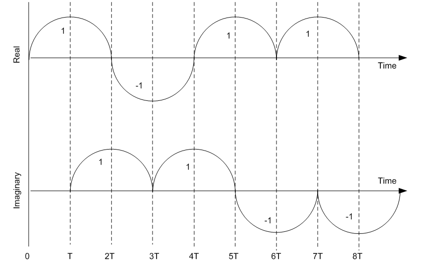
Real and imaginary components of baseband MSK with respect to time (T is the symbol period)

 

For another explanation of the same thing see http://www.dsplog.com/2009/06/16/msk-transmitter-receiver/ . This looks like two streams of data consisting of the 1s and -1s with one data stream offset by period T. We can decode each stream independently and then combine them later to produce the original data. However, we cannot simply send these 1s and -1s  symbols to the DDS chip directly, as the DDS chip for MSK will be expecting one of two frequencies which we denote with the + and - symbols. The following figure shows sending + then – and + then +, either of which produces a 1 to be sent in the imaginary stream as seen in the figure above.

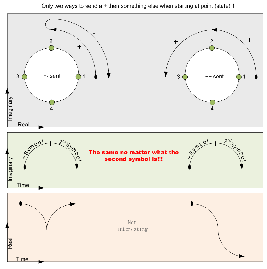
Using two symbols rather than one at a time

 

To convert the 1/-1s into +/- we can use an encoder. With a bit of thinking I realized that such an encoder could be written with the following trellis diagram. It’s almost a convolutional code but I don’t think it is as if you were to send a series of zeros the state oscillates between states three and four and output’s +-+-+-….

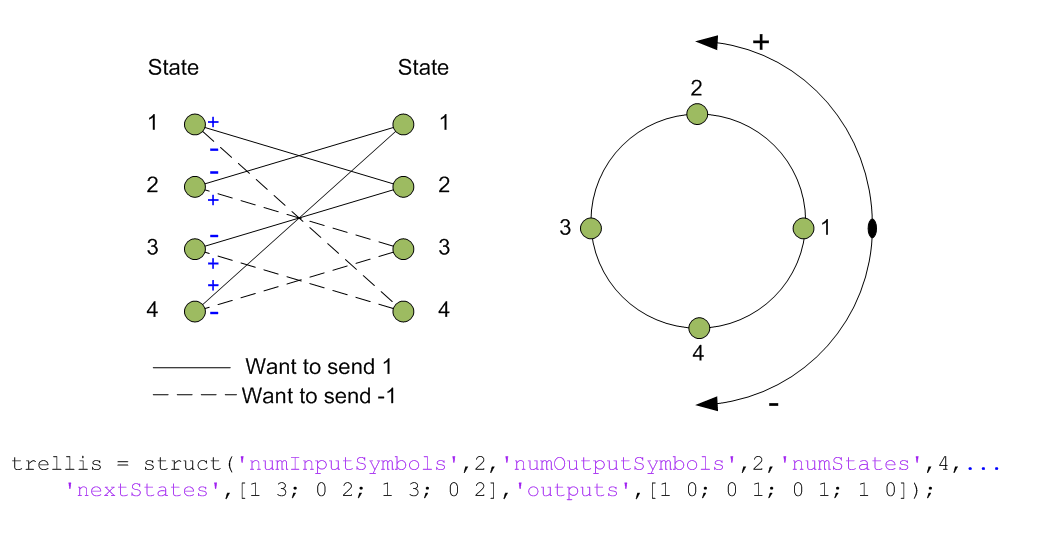
1/-1s to +/- encoder

 

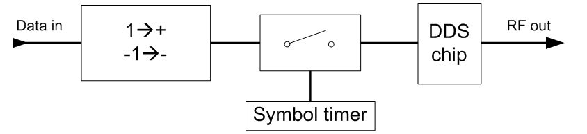
So, for example if you are at state 1 and you want to send a 1 then you output + and move to state 2. A block diagram of the MSK modulator with the DDS chip is depicted in the following figure.

 

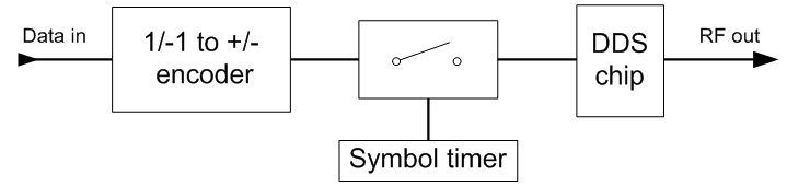
MSK Modulator block diagram

 

The two data streams in the very first image can be fed through a matched filter to maximize the probability of correct symbol identification. This matched filter performs correlation with the kernel that can be seen in the following figure.

 

Matched filter kernel

 

The kernel runs over each data stream, the points of the kernel are multiplied with the data stream piece by piece and added up to produce one value; the matched filter is a Finite Impulse Response (FIR) filter. The response of this matched filter for an MSK signal with correct carrier timing can be seen in the following figure.

 

 

Real and imaginary outputs from the matched filter for an MSK signal with correct carrier timing

 

 

As the two data streams are offset by a period T, if say the imaginary data stream is then delayed by a period T then the two data streams are synchronous with one another and we can then visualize the two data streams as if they will one. Such a data stream has four points and has a baud rate of 1/(2T). The following picture shows the procedure to obtain this from the passband.

 

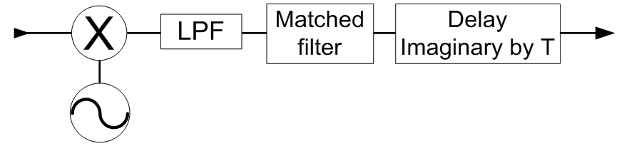
Obtaining the four point constellation data stream

 

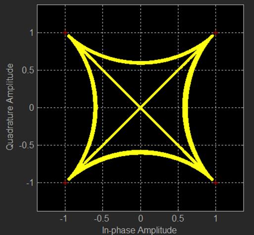
Once such a data stream is obtained, assuming perfect carrier frequency and phase (the squiggly thing in the previous figure which is the local oscillator matches that of the transmitter) we can produce a plot like the following. The figure shows all points possible with the vertices which are colored red being the location of the constellation points. If you sample at the correct time you will see four yellow points sitting on the red + marks; this contains the data of the two data streams and I call them “on points”.

 

The dreaded symbol timing and carrier tracking

 

Both symbol timing and carrier tracking must be performed by a demodulator in order to deal with the differences between the modulator and the demodulator. I find that when making a demodulator the symbol timing and carrier tracking are by far the hardest things and can seem to be as if these two aspects are all that a demodulator is. I was reluctant to read scholarly type papers as I find them quite often a waste of time to read, and I was reluctant to delve too much into the mathematics and instead see what I could do just by insight and observation. Pretty much all I read was the very useful blog http://www.dsplog.com/2009/06/16/msk-transmitter-receiver/ before attempting to make the demodulator, but this did not mention anything about symbol timing or carrier tracking. My first attempt at a demodulator I simply used a modified Gardner algorithm for symbol timing and used a fourth power of the constellation points as an error function to track the carrier. While this worked sort of okay with computer simulations with just Additive White Gaussian Noise (AWGN), the performance wasn’t outstanding and with real-life tests proved pretty dismal. There are many reasons why this did not work very well, firstly incorrect carrier alignment causes both a rotation of the points and a dispersion of the points as can be seen in the following figure so the fourth power trick is noisier than when using Phase Shift Keying (PSK), with the fourth power carrier cycle slips were fairly common in real-life tests as I had to keep the phase between -45° and +45° which is a fairly small range of angles, both the symbol timing and carrier timing were not separate and one could not be obtained without the other creating a bit of a catch 22 problem. My lesson learned here was while squaring things and putting things to the fourth power may be good for removing information but they add noise and shouldn’t be used to haphazardly.

 

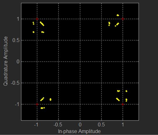
Correct symbol timing incorrect carrier timing

 

My next attempt at a demodulator was far more successful and I think very good. I wanted it to be more block orientated as programming in Matlab this way is easier. I also wanted that symbol timing was not reliant on carrier timing and vice versa. The idea with this demodulator was that small blocks of data after the matched filter were processed assuming a constant symbol rate and a fixed carrier rotation error. The carrier rotation error would be assumed to be unknown and all rotations between 0° and 90° would be examined to determine if any symbol oscillations could be detected. The rotation that had the greatest symbol oscillations would then be chosen as one of the two possible candidates for what was regarded as the real arm, the other being this rotation plus 90°. The phase of the symbol oscillations would either be the real arm or the imaginary arm, therefore symbol tracking could be used to determine if the found carrier rotation was for the real or imaginary arm and hence resolve the carrier offset to between -90° and +90° thus reducing the possibility of cycle slips compared to the fourth power method. That is my idea for carrier and symbol timing, so let’s delve into greater detail.

 

Carrier and symbol timing estimations

 

A small block of data is obtained after the matched filter assuming a fixed carrier rotation and symbol timing. This block is rotated first 0° then 1° and so on up to 89°, each of these rotations is then squared and the real component examined for oscillations that happen due to the symbol rate. If there was no carrier rotation then for the block that was rotated 0°, the real component of this block would contain one of the streams of data and can be seen in the following figure in blue while that of squaring each item in the block and then taking the real component of this can be seen in the following figure in red.

 

 

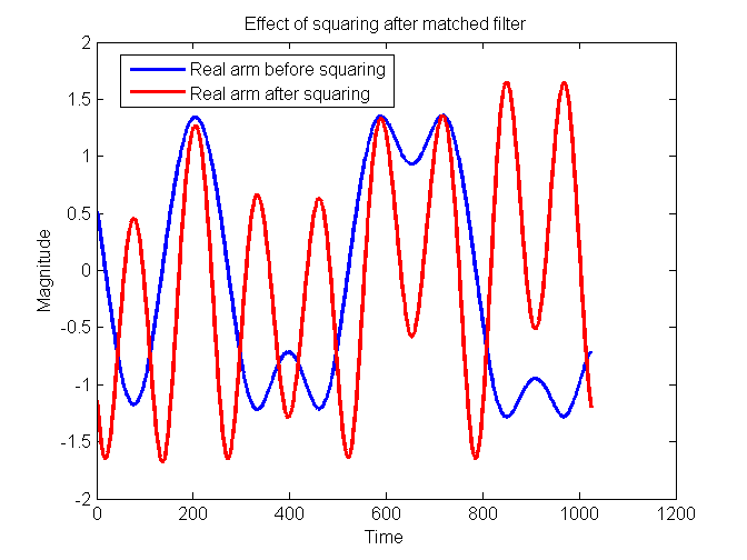
Effect of squaring after the matched filter

 

It can be seen that the peaks of the red plot match the sampling time for this particular stream (or arm) of MSK data. As each stream is sent at a rate of 1/(2T) where T is the symbol period, a Discrete Fourier Transform (DFT) of 1/(2T) will supply us with both an estimate of the amount of the signal strength for a particular rotation and the symbol phase so as to inform us when to be sampling. The rotation that causes the greatest signal strength will be a rotation that aligns one of the MSK data streams along the real axis, this is the rotation we are looking for. A block diagram of the procedure is shown in the following figure.

 

 

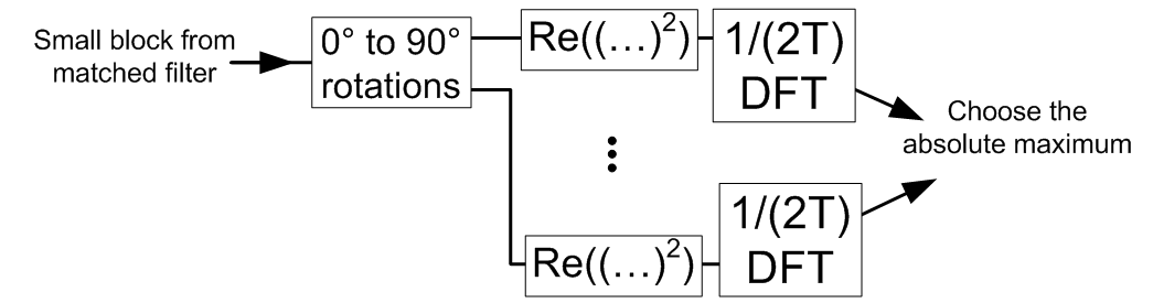
First step in finding carrier rotation and symbol timing

 

 

A Matlab code snippet can be seen as follows where sig2 is the small block of data while the carrier rotation estimate is rotationest and the symbol phase timing estimate is symboltimginphaseest.

 

First step in finding carrier rotation and symbol timing code snippet

 

This is only the first step in estimating carrier phase and symbol timing. This is because we may have found the carrier rotation of the wrong MSK data stream and the returned symbol timing phase estimate may also be for the wrong MSK data stream. To solve this problem we randomly track one of the MSK data streams and perform a judgment call as to which MSK data stream the previous step has given us. As the symbol timing phases of the two MSK data streams are 180° out of phase, if the returned symbol timing phase estimate given to us from the previous step is more than 90° out from where we believe the current symbol timing to be, we performed a judgment call that indeed we have been given the wrong MSK data stream and that the symbol phase timing estimate is 180° out while the carrier rotation is out by 90°. A GIF animation of both the symbol timing phase estimate returned from the previous step and the symbol timing phase tracking can be seen in the following figure. The inner dots represent the symbol timing while the outer ones represent the symbol timing phase estimate returned from the previous step.

 

 

Symbol timing tracking given symbol timing phase estimate from the previous step

 

A Matlab code snippet of the symbol timing tracking and reduction of carrier phase ambiguity can be seen in the following code snippet where hSymTracker.Phase is the tracked symbol timing phase estimate and carriererror the carrier rotation error with reduced ambiguity to between -90° and +90°.

 

Second step in finding carrier rotation and symbol timing code snippet

 

Next the carrier of the receiver has to be adjusted using the estimate from the previous step so as the receiver maintains a coherent oscillator with respect to the modulator’s oscillator. This is simply done by gently adjusting both the phase and the frequency of the receiver as can be seen in the following Matlab code snippet.

 

Carrier phase and frequency adjustment given carrier error estimate

 

However, this carrier tracking requires a very good initial frequency estimate else it won’t work. Because of this a coarse frequency estimate within a few hertz is needed for carrier tracking to work. This coarse frequency estimate I obtained by examining the spectral peaks when the baseband is squared. If you square the baseband signal and take Fourier transform of it you obtain something like the following.

 

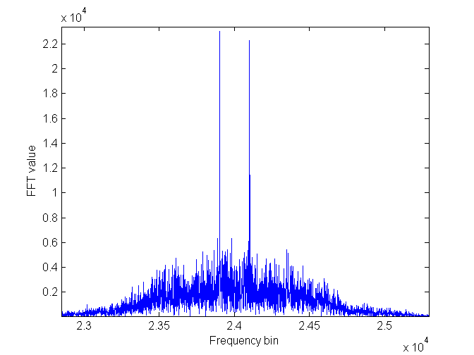
FFT of the baseband squared for coarse frequency estimation

 

The two spectral peaks correspond to the two frequencies used to make the MSK. The average of these two frequencies is that of the transmitter and is the frequency we wish the receiver to be at. The following code snippet takes the baseband signal (rawt) and estimates the transmitter’s frequency as hPFOd.FrequencyOffset.

 

Coarse frequency estimate and correction if needed

 

Putting everything together the demodulator can be depicted as follows.

 

  
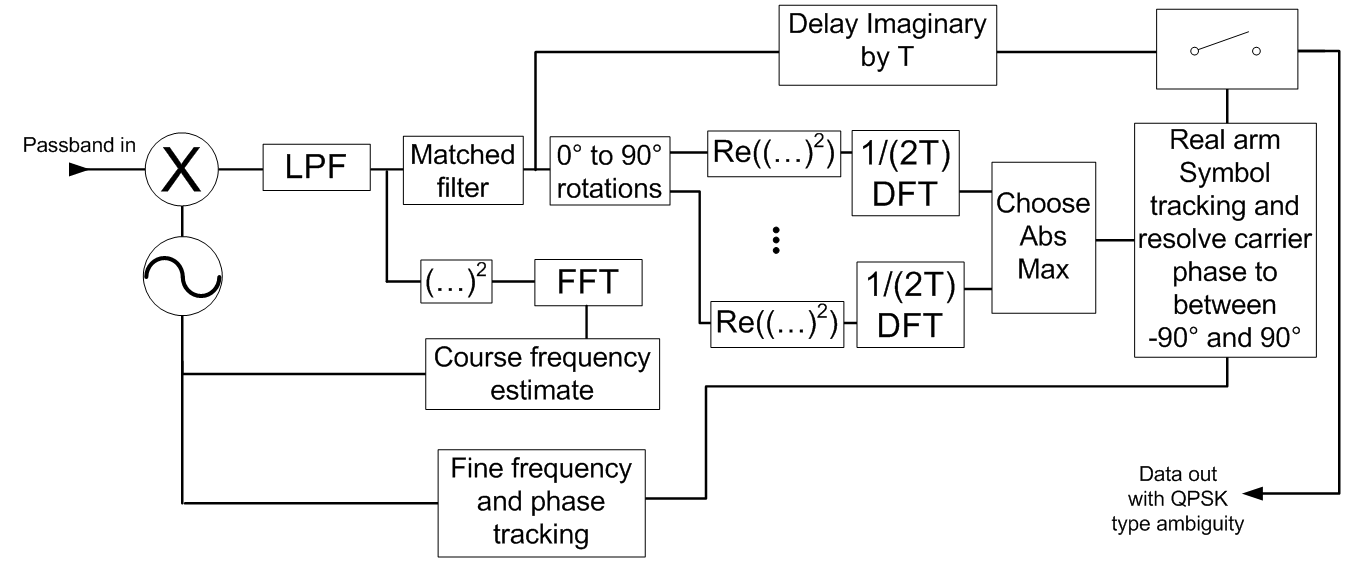
MSK Demodulator block diagram

 

 

This type of demodulator is a coherent demodulator and does not use differential encoding. Without using differential encoding there is an ambiguity in the final data points where the rotation can be either 0°, 90°, 180°, or 270°. With respect to Bit Error Rate (BER) in the presence of AWGN this type of demodulator performs slightly better than if differential encoding was used which in turn performs slightly better than an incoherent demodulator with differential encoding.

The following figure shows a Matlab simulation of the demodulator with initially an incorrect symbol rate and carrier frequency and a certain amount of AWGN. After a few seconds to allow the demodulator to acquire the signal the demodulated data was recorded and this continued for approximately 300,000 bits. The final ambiguity was resolved by taking the lowest BER and plotted in the graph below along with theoretical plots for incoherent Differential Binary Phase Shift Keying (DBPSK), coherent Differentially Encoded Binary Phase Shift Keying (DE-BPSK) and coherent Binary Phase Shift Keying (BPSK).

 

 

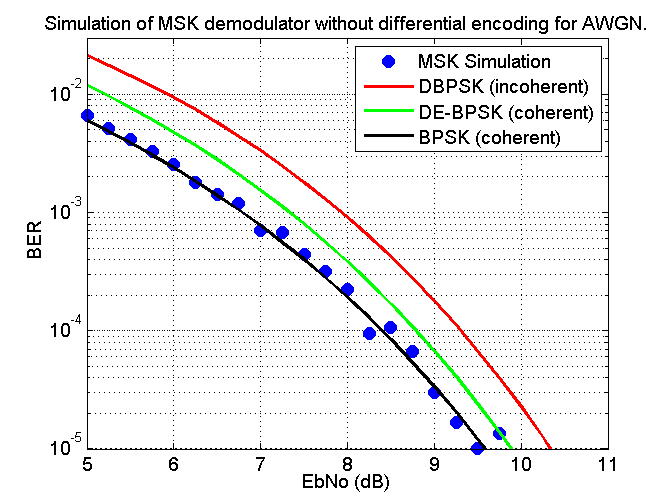
Simulation of MSK demodulator without differential encoding for AWGN

 

The reason for including the theoretical plots is to show that this form of MSK demodulator has the same performance in the presence of AWGN as a coherent BPSK demodulator. The incoherent DBPSK plot (red plot) I believe is how most if not all PSK31 demodulators work.

 

Differential encoding

 

I wanted to implement differential encoding so I did not have to worry about resolving the final ambiguity and instead take the small performance hit as seen in the previous figure and move to the green plot. Without my so-called 1/-1s to +/- encoder the modem naturally perform some sort differential encoding. So I tried to see if I could gain some understanding on how this naturally occurring differential encoding happens.

For the 1/-1s to +/- encoder (the encoder), if we represent – and + by 0 and 1 respectively and -1 and 1 by 0 and 1 respectively this encoder can be depicted as follows. That it seems to need an oscillator is the reason why I think it’s not convolutional encoder. Due to the oscillator any datastream that goes in can be mapped to one of two output data streams. In addition any input bit can only affect the current output bit and the next output bit. It also has a rate of one. If it wasn’t for the oscillator it would look like the standard differential decoder as seen on the page https://en.wikipedia.org/wiki/Differential_coding .

 

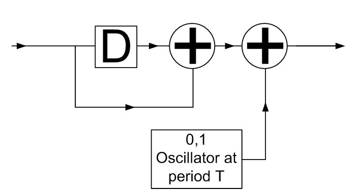
The encoder

 

To create differential encoding we now remove the original encoder so the modulator looks like the following figure.

 

 

Modulator with differential encoding

 

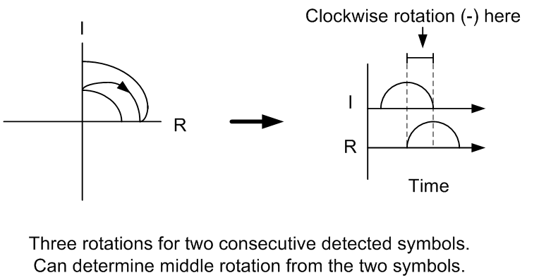
With the the -1s and 1s we wish to send now mapped to the – and + quarter rotations respectively, it is possible to detect the direction of rotation of one of the three rotations when given two consecutive received symbols. As an example if we start on the real axis and send the rotations +-+ we will receive first a 1 on the imaginary arm then a one on the real arm; in this case the middle rotation can be determined to be a - from just the two received symbols. Visually this process can be seen in the following figure.

 

 

The first and the third rotations do not affect the middle rotation. Going through all eight possibilities we obtain the following mapping where  represent the consecutively received symbols a and b from the imaginary and real arms respectively. Likewise  the consecutively received symbols b and a from the real and imaginary arms respectively.

 

 

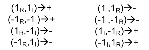
Mapping of the eight possibilities for two consecutive symbols

 

This can be drawn as a trellis diagram as follows where the first set of transitions are due to the received imaginary symbol, while the second set of transitions are due to the received real symbol.

 

 

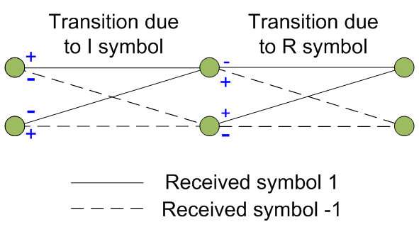
Trellis diagram for the mapping from symbols to rotations

 

Noticeably there is a similarity between the two sets of transitions, where the second set of transitions the output has simply been inverted compared to the first. This inversion allows an obvious implementation simplification by simply inverting the output of the trellis diagram if the transition is due to an imaginary symbol and removing the distinction between transitions due to the imaginary symbol and ones due to the real symbol. The transitions due to the real symbol is simply a standard differential decoder, therefore an implementation of the above trellis diagram can be given as follows where – and + are mapped to 0 and 1 respectively while -1 and 1 are mapped to 0 and 1 respectively.

 

 

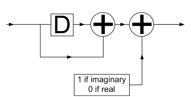
Implementation of mapping symbols to rotations

 

As can be seen this is almost identical to what the encoder was except the oscillator has been replaced with something that is linked to whether or not an imaginary symbol or real symbol is being processed.

 

For my implementation of the demodulator I always delay the imaginary arm by T meaning the imaginary component has to be processed before the real component; this being the case the following Matlab code snippet is enough to allow the demodulator to decode varicode symbols that have been sent via the naturally occurring differential encoding that gets performed by the modulator when not using the encoder. I’m always amazed how much thinking goes into figuring out something that in the end look so simple.

 

Matlab code snippet for decoding differentially encoded MSK

 

Testing differential encoding

 

Now we have a method of performing differential encoding and decoding using MSK we can check the performance matches that with what should be expected. The following figure was created using the same demodulator as previously been described except with the removal of the encoder on the modulator and with the additional implementation of the differential decoder as just described.

 

 

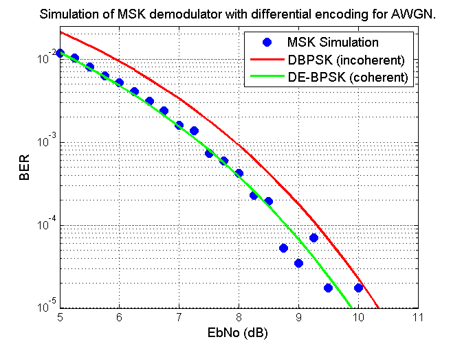
Simulation of MSK demodulator with differential encoding for AWGN

 

As can be seen the results are very similar to coherent differentially encoded binary phase shift keying; we take a hit of approximately half a decibel as expected but gain the benefit of not having to resolve any ambiguities. For the remainder of this document I solely use this method of differential encoding. In addition I use varicode as implemented in PSK31 to transmit text through the modem.

 

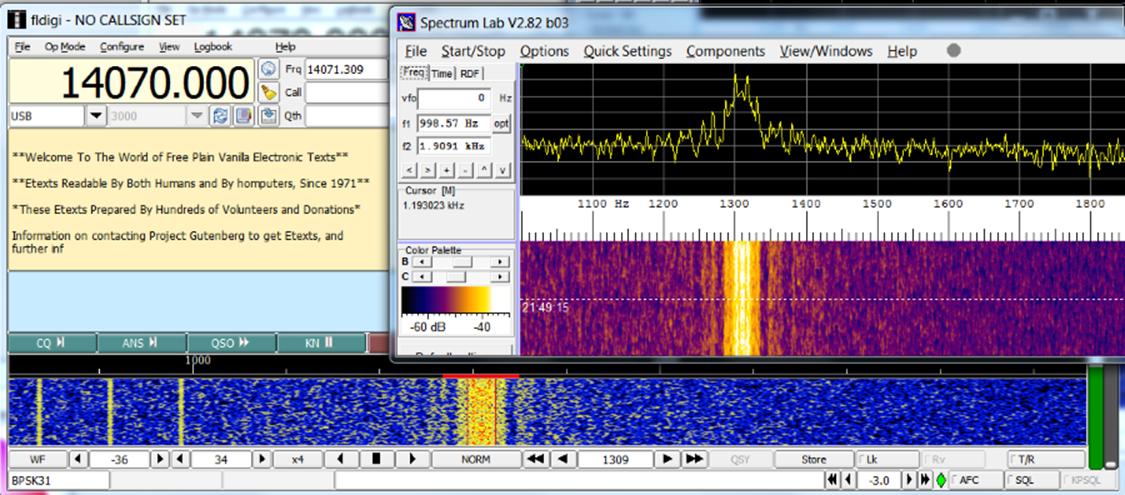
Almost real life testing

 

Before commencing any real life tests using physical external hardware I chose to use spectrum lab and the digimode component that it has to create varicode differential encoded MSK for my Matlab implementation to decode. To get spectrum lab to modulate using MSK I used the following settings.

 

 

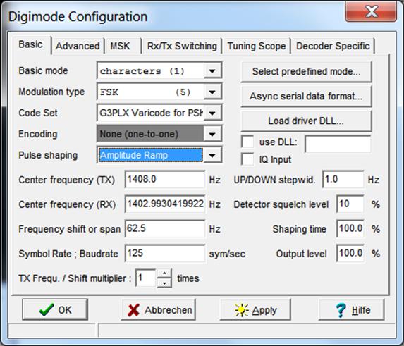
Settings used for spectrum lab to modulate MSK

 

Spectrum lab uses a continuous phase frequency shift keying so the previous settings will be able to produce MSK at 125 bps. The following figure shows my Matlab implementation decoding the signal along with the spectrum of the MSK signal.

 

 

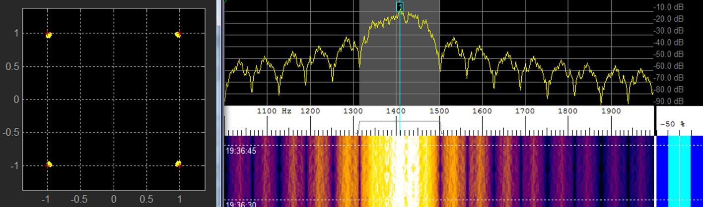
Matlab decoding Spectrum lab MSK signal: no filtering.

 

In the next figure I have filtered everything beyond the first nulls of the signal with little noticeable effect on the demodulator.

 

 

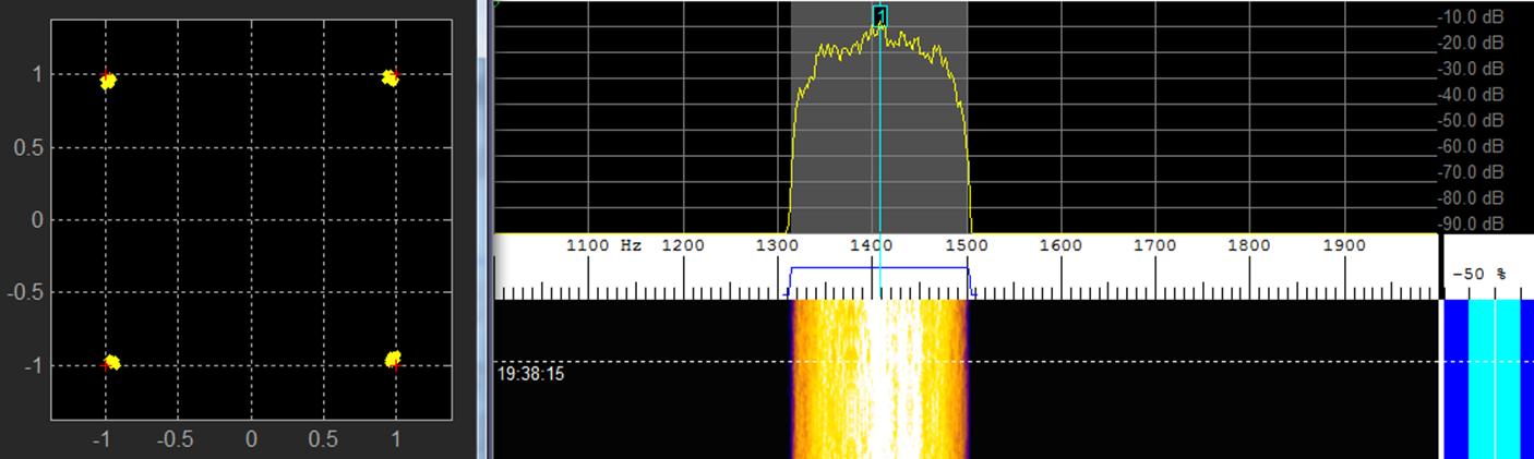
Matlab decoding spectrum lab MSK signal: filtering beyond first nulls

 

The text was decoded perfectly both times.

 

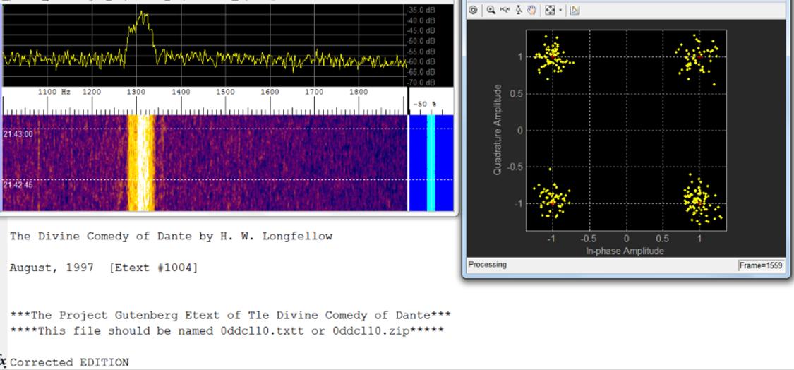
Initial real life testing

 

A laptop was setup with the Arduino and the DDS chip as used in JDDS . A program was written in Qt to cause the DDS chip to produce a MSK modulation at 125 Baud that was encoded with English text. An RTL-SDR dongle was attached to another computer and SRD# used to receive the RF signal from the DDS chip. The two computers were separated by less than a meter. The following screenshot shows the computer with the RTL-SDR dongle demodulating and decoding the English text.

 

Demodulating MSK sent over RF via the DDS chip

 

The top left shows the received frequency spectrum, the top right is the four-point constellation, and the bottom is the text as it is being received.

I used a three second buffer for the coarse frequency estimation and a block by block processing of 128 ms where any remaining carrier offset was compensated for. This produced some jitter of the points but removed any bias in the constellation and speed up the time required until readable text was seen. This meant after the three seconds to estimate a course frequency, for a reasonably strong signal, readable text was seen after a hundred milliseconds or so.

Generally things performed as expected and I was very pleased with the performance of the demodulator. From a cold computer once the power had been applied to the DDS chip, the DDS chip’s local oscillator would be somewhat erratic initially and whose frequency would tend to decrease as the oscillator warmed up; this can be seen in the previous figure where the frequency is dropping ever so slightly. After 10 minutes the DDS chip’s oscillator would stabilize. During the period when the oscillator was erratic, the demodulator still had no problem maintaining correct carrier timing.

 

Weaker real-life signal test

 

Reducing the RTL dongle RF amplifier gain and reducing its antenna I went about seeing how low the signal could be before demodulator would perform poorly. I use the same 125 Baud rate as before. The figure below shows about as far as I could push it and there are considerable numbers of errors in the received text. The signal was so weak that I had difficulty hearing it.

 

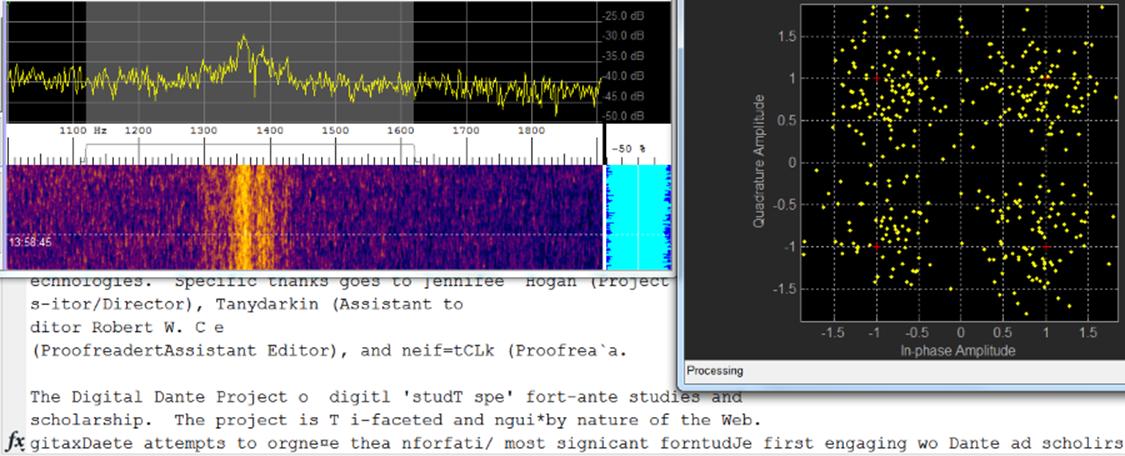
MSK demodulation with a very weak signal

 

26 meter test of MSK at 50 Baud and PSK31

 

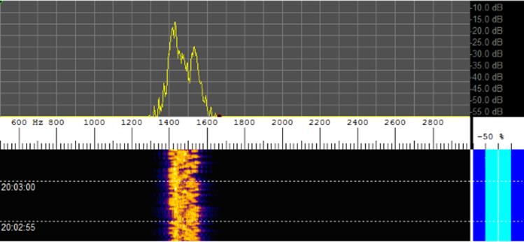
I placed the DDS chip 26 meters away in the garage which was clad in metal and separated by three walls. I put a small piece of wire on the DDS chip. I performed two tests, one where the DDS chip produced an MSK signal and another where it produced an unfiltered DBPSK signal. The MSK was at 50 Baud and the DBPSK was at 31.25 Baud. 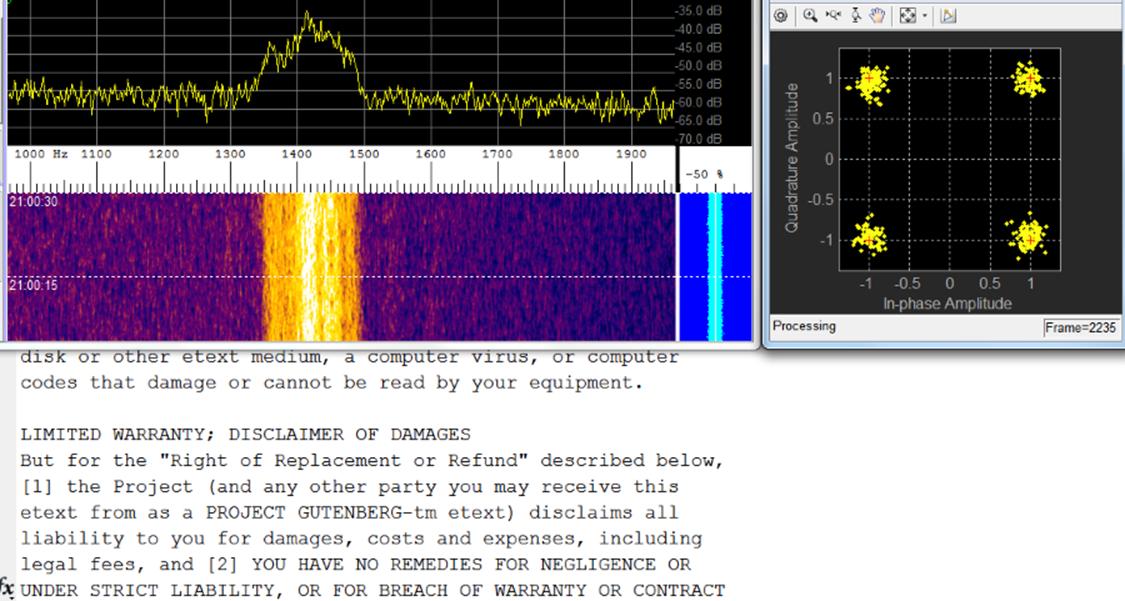Below is a screenshot of the received spectrum, constellation and the decoded text using the described demodulator for the MSK test.

 

 

DDS chip producing MSK at 50 Baud. 26 meters

 

The next screenshot is of the DBPSK test and comprises of the received spectrum (Spectrum lab’s scale is the same as that of the MSK test) as well as the decoded text using Fldigi as the DBPSK demodulator.

 

DDS chip producing DBPSK at 31.25 Baud (like PSK31). 26 meters

 

For both tests the signals were good. I saw one incorrect character shortly after acquisition during the MSK test, and another incorrect character for the DBPSK test which can be seen in the previous figure. The first one or two side lobes of the DBPSK test can be clearly seen while it is hard to tell if any side lobes from the MSK signal can be seen. This brings me to one of the reasons why I’m interested in MSK for the DDS chip rather than BPSK.

Spectral components of unfiltered BPSK and MSK

 

The DDS chip is unable to produce filtered BPSK as it stands. Even if it could it would require a linear amplifier which is not something I like as linear amplifies are more complicated and less power efficient. Therefore it must produce unfiltered BPSK. Connecting the DDS chip directly to the soundcard I obtained the following spectral plot when the DDS chip was modulating using BPSK at 125 Baud.

 

 

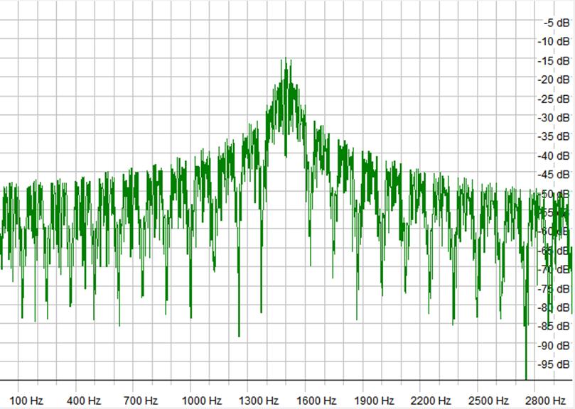
Spectral plot of BPSK at 125 Baud

 

I then averaged the spectral components over a longer period of time and calculated approximately the peak of each side lobe as can be seen in the following figure.

 

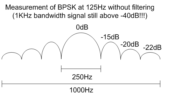
As a rule of thumb I consider as a minimum, the maximum out of band power peak must be at least 40 dB less than the maximum in band power peak. From the previous figure even with approximately a 3 kHz bandwidth this is not enough bandwidth to satisfy this rule of thumb. There is approximately a 30 dB difference between the center of the plot and either of the sides of the plot. As the bit rate is only 125 bits per second this is very spectrally inefficient at less than 0.04 b/s/Hz; you would not want to transmit this signal in real life.

I then performed the same test but used MSK to modulate the DDS chip at 125 Baud and obtained the following spectral plot.

 

 

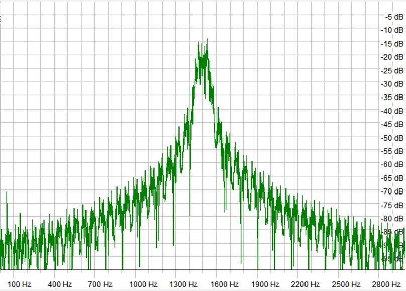
Spectral plot of MSK at 125 Baud

 

This again averaging the spectral components over a longer period of time and calculating the approximate peak of each side lobe I produced the following figure.

 

 

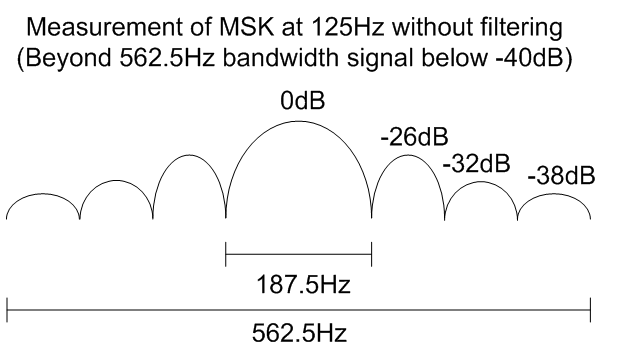
This time the falloff in power has been improved greatly. A bandwidth of approximately 562.5 Hz (4.5 times the bit rate) would satisfy my 40 dB rule of thumb. This produces a spectral efficiency of approximately 0.22 b/s/Hz. This is not a great spectral efficiency but it’s a lot better than BPSK and would be fine for slow bit rate applications. In addition, as MSK has a constant envelope it is suitable for amplification using nonlinear amplifies which are simple to make and power efficient.

 

The other reason I’m interested in MSK rather than BPSK

 

16MSK is a generalization of MSK to 16 frequencies rather than two. Like MSK the frequencies and the Baud rate are related so if you are on the real axis any symbol will move you to the imaginary axis and vice versa. This means if a symbol has a period of T, then the 16 frequencies used for 16MSK are -15T/4, -13T/4, -11T/4, -9T/4, -7T/4, -5T/4, -3T/4, -T/4, +T/4, +3T/4, +5T/4, +7T/4, +9T/4, +11T/4, +13T/4, +15T/4. I have no way of demodulating 16MSK at the moment but I can produce it easily enough using the DDS chip as can be seen in the following figure.

 

16MSK at 100 b/s

 

Matlab seems to call what I’ve been referring to as MSK as 2CPFSK with modulation index 0.5, and 16MSK as 16CPFSK with modulation index 0.5. Using Matlab’s “bertool”, I plotted what Matlab considers to be the theoretical BER versus EbNo curves for BPSK, 2CPFSK and 16CPFSK where the modulation indices of the two CPFSK modulation schemes where 0.5; this plot can be seen in the figure below where BPSK curve cannot be seen because it lies under the 2CPFSK curve. If this is true, Matlab is saying that a gain of 6 dB can be achieved by using 16CPFSK rather than 2CPFSK or BPSK; that’s equivalent to saying that you can get away with using only a quarter of the power you would normally use to transmit a signal using say BPSK or MSK.

 

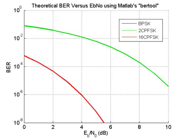
Theoretical BER Versus EbNo using Matlab’s “bertool”
2CPFSK and 16CPFSK have modulation indices of 0.5

 

This extremely large gain is very attractive and is the other reason I’m interested in MSK. I’m interested in extending the demodulator I’ve implemented to 16MSK. This however is for another day.

 

The DDS chip as a modulator

 

Using the DDS chip is a modulator was pretty easy. It used my SLIP library and a simple Arduino code. A short video clip of me using it to send both DBPSK and MSK is given in the following video clip.

 

 

Sneding DBPSK and MSK using the DDS chip

 

The source code for both the PC and the Arduino are given below. It could do with a tidy up but it’s what I’ve been using.

 

DDS chip modulator download:

 

Source code for the Matlab MSK demodulator

 

The Matlab source code for the MSK demodulator is given below. Once again it is something that could do with a tidy up, but it works.

 

MSK demodulator Matlab source code download:

 

Cross-platfrom stand alone binary

 

The Matlab demodulator as described on this page has now been ported to Qt C++. This allows the demodulator to be run without the need for Matlab. See the JMSK main page for this application.

 

 

Jonti 2015
Home