The Softrock Lite II and WSPR
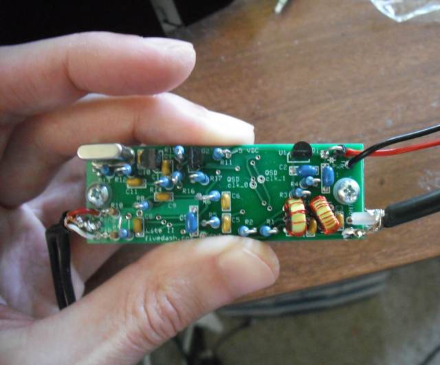
A few weeks ago I bought a Softrock Lite II kit. Initially I didn't know how I can cope with being limited to such a small amount of bandwidth. The bandwidth that you can receive is limited by the sample rate of your soundcard so a 96khz limits you to around 90 kHz bandwidth. But in retrospect having such a limited bandwidth I think is a positive; you focus on the small amount of bandwidth without rushing all over the place hoping to find a strong signal somewhere. This way you can start tackling some weak signals in a surprising what is actually out there.
The Softrock lite II it is amazing. It's really sensitive, really stable, and does a great job at rejecting all the incredibly high power broadcast signals out there. I would highly recommend getting one of these little devices, in way outperformed my expectations of it.
To begin with you have to choose your bandwidth so I chose the 20 m band. When I run my computer on Linux I can get my soundcard working at 192khz which means I can get over 14,130khz.
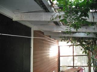
My aerial I just used a dipole-ish antenna along the veranda. I couldn't run it straight so it has a 90° dogleg in it, that's why I say ish.
On the lower part of the 20 m band that the soft rock can do is the Morse code people. If your sound card can only go up to 96khz you wouldn't get a great deal more than a Morse code people. You'll still be able to get an interesting weak signal digital mode called JT65 and a few other bits and pieces like some rtty. But for me I do like having the 192khz sample rate although it doesn't seem to work on Windows.
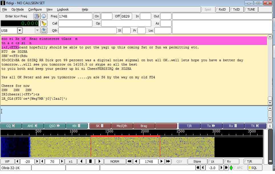
Passed the Morse code people you start getting the digital modes. I like the the Olivia mode as it has great error correction which means its easy to copy unlike rtty.
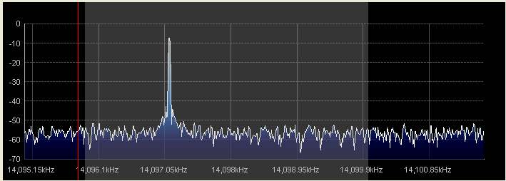
Cruelty, just ever so slightly above what a 96000khz can can do is one really fascinating mode called WSPR around 14,097.1khz. you may not even be able to hear anything there. It uses about 200 Hz of bandwidth so is fairly compact. Running the sound into the WSPR decoded you get something like the following.
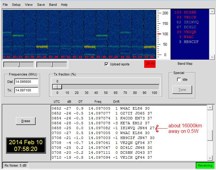
There are lots of transmitters over the world sending their call sign where they are in the world and how much power the transmitting with. In the previous screenshot I received some one from Italy around 16,000 km away on only 0.5W. Which is staggering when you consider some hams put out 1kW to get the same distance.
Making a signal
The protocol says that you transmit at 1 second past on even minutes. You transmit 160 so symbols of 4FSK that takes about two minutes, so it's a slow throughput. It uses 6 Hz of bandwidth.
I already had a couple of the $5 DDS modules from ebay lying around. They are AD9850 chips.
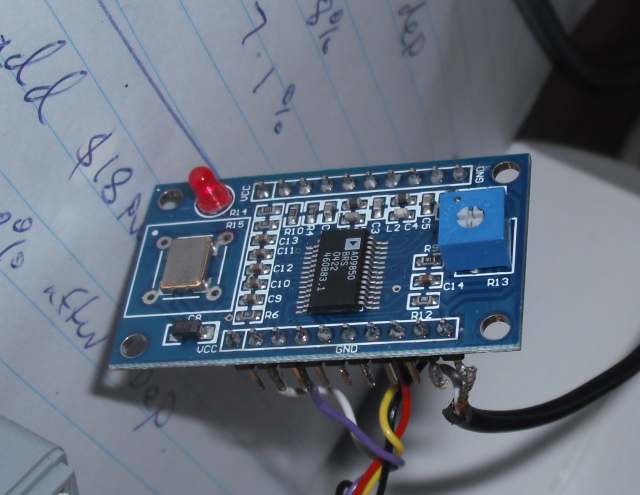
I've had a look at the signal these produce and compared them to the GPS frequency stability. I am somewhat disappointed with there stability and their phase jitter.
I found out I had to run them at 3.3 V as the oscillator in mine has the maximum voltage of something like 4 V and when I have it running at 5 V after a few minutes the oscillator got really hot and the signal the DDS chip produced went haywire.
Of course to control a DDS chip you need a microprocessor so I connected it to a arduino uno; the three signal wires I ran through 470ohm resistors.
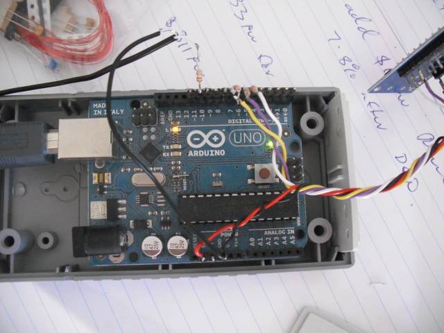
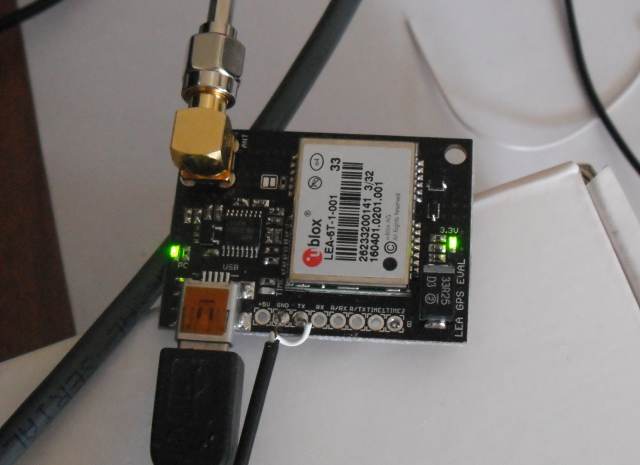
Keeping time also important for WSPR and easiest way to do this is to use any old GPS receiver and connect the tx out of the GPS receiver through a 470ohm resistor to the arduino.
Looking at the DDS module it seemed there were two analog outputs, I couldn't find any square wave output from the pins. The two analog ones were complimentary so when one would be at 1V the other one would be at 0 V and vice versa.
The next step was to amplify and filter the signal.
I already had a board lying that almost had all the makings of an amplifier. So with a few adding and changing of components a 200mW amplify was born.
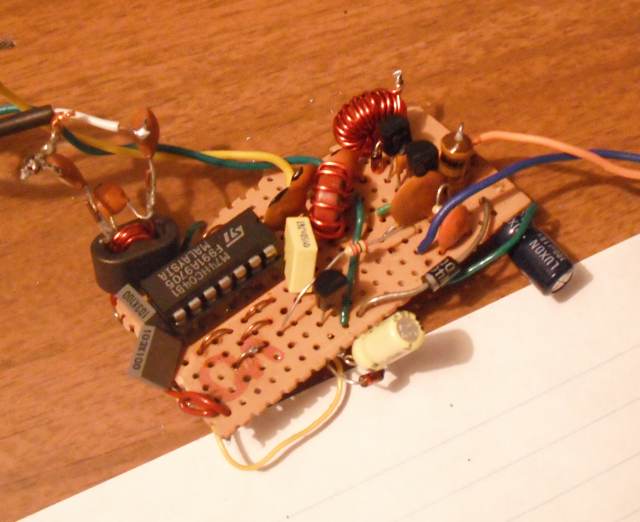
Below are the actual components I used.
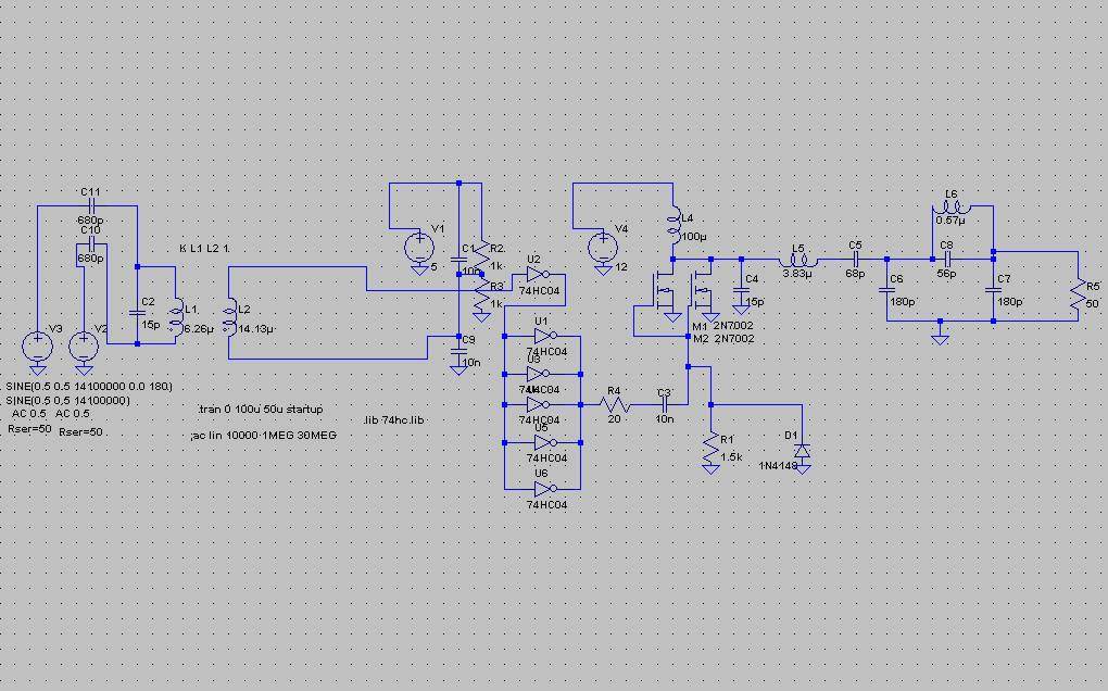
Fets acording to ltspice. What?? this is not right. The current through the fet
is not stopping when the fet turns off and current is to late. Does LtSpice not
simulate 2n700 correctly or does this actually happen in real life?
In real life the efficiency of the amplifier turn out low. The efficiency including the linear 5v regulator for the 74hc04 from a 12v input was about 27%. Ideally over 60% efficiency would have been preferred.
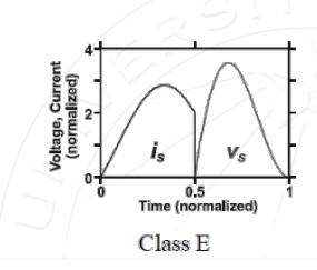
Fets as they are supposed to be.
Changing to BS170 fets and adjusting C4 and L5 according to ltspice. Seems
Now current is zero more or less when voltage is non zero; this is right.
Although it is supposed to be a class E amplifier it's not efficient as it should be, it uses too much power for an output of only 200 mW final output. according to ltspice the 2N7000 transistors don't seem to make the waveforms that they should, the BS170 transistors on the other hand seem to; I don't know what this is about. Is it a problem with the way Ltspice's models the BS170 and the 2N7000?. it's also a bit of a hassle because the driving circuit has to have 5V while the two FETs require more like 12 V. You also don't need two fets for 200mW one would be plenty. the funny values for the transformer are due to what I actually measured when I made the 1:2 transformer. So if I was doing this again I'd change things, I'd change the driving circuit, use BS170 as and recalculate the class E amplifier part so it used only one fet. http://www.wa0itp.com/class%20e%20design.html gives you a convenient way of designing class E amplifies.
According to LTSpice the final signal should look like the following with at least 50 dB attenuation.
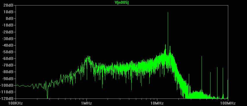
Close up in real life we get the following
The Micro
Then comes the programming of the microprocessor.
Although I don't like Arduino as I find it hides a lot of things under the hood it certainly does make a very fast prototyping platform for ideas.
So I gathered the following libraries and imported them into the Arduino IDE
TinyGPS
Time
Timer1
AD9850
SoftwareSerial
And then wrote the following code
The code uses a hard coded WSPR message to send. to generate the desired message I used this program http://physics.princeton.edu/pulsar/K1JT/WSPR.EXE . when typing something like the following the second column of text that is outputted refers to what symbol is to be used.
"wspr Tx 0 0.0015 0 N0CALL AB12 23 11"
Gathering these all up and putting them into something that c++ can read results in something like
byte WSPR_DATA[] =
{3,3,2,0,0,2,2,0,1,0,2,2,1,1,3,2,2,2,1,0,0,1,2,1,3,3,3,2,0,0,0,2,0,0,1,0,0,1,2,3,2,2,2,2,0,0,3,0,1,3,2,2,1,
3,0,1,2,2,2,1,3,0,3,2,2,0,2,1,1,2,3,2,3,2,1,0,3,2,2,3,2,2,1,0,1,3,2,2,0,1,3,2,1,2,1,0,2,2,1,0,2,0,0,2,1,2,2,1,0,0,1,3,1,0,1,3,0,0,3,
1,2,3,0,2,2,1,1,3,2,0,2,2,2,1,0,3,2,0,3,3,0,0,2,0,2,0,0,3,3,0,3,2,1,3,2,0,2,1,3,0,2,0};
This has to be put into the program before uploading to the arduino.
So there's no real time modification to the WSPR message sent but everything else can be controlled in real time via the usb serial port of the arduino.
Upon connecting to the arduino you get something like the following interface.
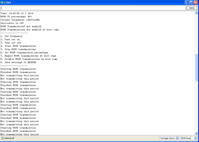
You can do things like set the frequency, the transmission percentage and enabling and disabling messages to be sent when the arduno unit is powered on. changes you make can be saved to the eeprom. You can also turn on and off the DDS so you can create an arbitrary frequency for testing purposes.
Randomness of WSPR transmissions
With WSPR transmissions each slot is two minutes long. Say you want to transmit in 33% of the slots. This means you have to decide which slot you transmit in and which ones you do not with the resulting percentage of slots used by you equating to 33% of all slots.
There are two extreme ways you could do this. Firstly you could randomly take numbers between zero and 99 inclusive and when you get a number less than 33 you transmit in the slot. The other way you could do it is to systematically take every third slot. Both ways you would be taking 33% of the slots. the difference in these two methods is the first random method produces clumping where at times you will consecutively take many timeslots while at other times you'll miss many more than just two in a row. The second method you will never take two consecutive time slots everything is spaced out nicely but there is no randomness in the pattern.
If we represent taking a transmission slot with the number one and not taking one by the number zero we can see these two methods in the following sequence of numbers.
If we just use the random method as an example we could get the following
sequence of numbers.
1,0,0,0,0,0,0,0,0,0,0,0,0,1,1,1,1,0,1,0,0,0,1,0,1,0,1,0,0,1,0,1,0,0,1,1,0,1,0,0,0,1,0,0,0,0,1,0,1,0,0,0,0,0,1,1,0
If on the other hand we use the sparsely spaced repeating pattern method we
can only get the following set of numbers.
1,0,0,1,0,0,1,0,0,1,0,0,1,0,0,1,0,0,1,0,0,1,0,0,1,0,0,1,0,0,1,0,0,1,0,0,1,0,0,1,0,0,1,0,0,1,0,0,1,0,0,1,0,0,1,0,0
Both sequences have about 33% of ones.
From these two extremes the next thing that I wondered if there was something in between the two extremes. So I thought make a sparsely spaced repeating pattern as in the second method and then for a certain percentage of each slots replace the slot with a number from the first method. As this may change the percentage of ones, monitor the percentage of ones and change the underlying percentage of the sparsely spaced repeating pattern such that the final number of ones is still 33%.
While this sounds really confusing its actually very easy and written in C++ code it can be expressed as follows.
As you can see it's been three basic steps. Firstly use your knowledge about the current percentage of ones to choose whether or not a slot (sig) is a one or zero. secondly each slot has a probability of being replaced with random data that still does 33%. Finally track the approximate percentage of ones which is required for making the sparsely spaced repeating pattern.
So what does it look like? Well the first two sequences of numbers I showed you above simply came for me plugging in the the perturbation percentage firstly at 100% and then secondly at 0%.
Taking 10,000 numbers with the perturbation percentage at 100%, there were 32% ones, and at one point there was eight ones in a row. Doing the same but with the perturbation percentage of zero, there were 33% ones and there was never more than one one in a row.
| Perturbation percentage | percentage of ones | maximum number of ones in a row |
| 0 | 33 | 1 |
| 10 | 33 | 3 |
| 20 | 33 | 4 |
| 30 | 33 | 4 |
| 40 | 33 | 5 |
| 50 | 33 | 5 |
| 60 | 33 | 5 |
| 70 | 33 | 6 |
| 80 | 34 | 6 |
| 90 | 33 | 7 |
| 100 | 32 | 8 |
Generally the percentage of ones where very close to 33%. For higher perturbation percentages they started to vary little more than a low values.
Graphing these results there is clearly some sort of monotonic increasing relationship.
So this gives you a way to limit the maximum number of consecutive timeslots taken at the expense of some randomness.
Why not use a perturbation percentage of zero to avoid clumping transmissions together? well this would produce no randomness and if another transmitter was using the same pattern there is a 33% possibility that you will both be transmitting at the same time and never be able to hear one another. So we do need randomness and hence the perturbation percentage greater than zero.
Perturbation percentages too high however will cause clumping and for something like WSPR if you haven't transmitted for a quarter of an hour when you want to be transmitting a third time you might miss good ionospheric conditions for long-distance communication.
As for what the optimum perturbation percentage to use is, I'll leave that for someone else to do.
In the Arduino code I set it to 10%.
You might also want to add some random frequency hopping to the code for some more collision avoidance.
Power on
I was blown away with what sort of distance you can get with 200 mW. A few 1000km are typical most of the time and at some times of the day distances over 10,000km happen.
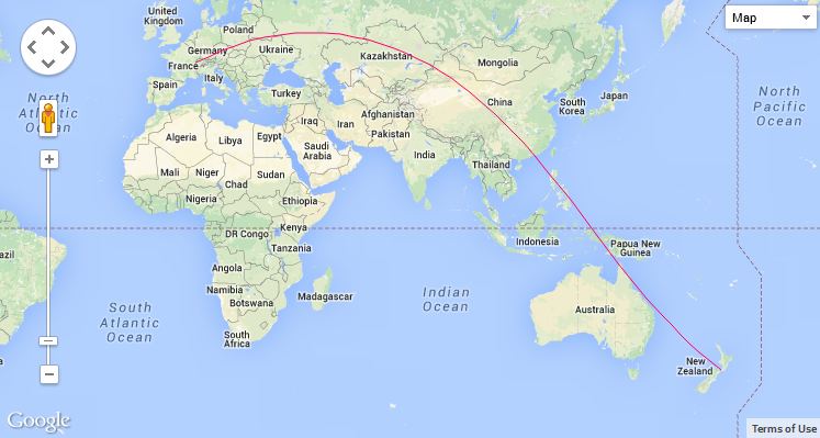
Looking at who had heard the signal, someone received it at over 18800km (a later day I saw someone received the signal at over 19700km). That's just about as far as any two points on the planet can be. That type of distance is not a common event though. Events like this seem to be very location specific and seem to almost link two small locations in the world together; this particular one lasted for about two hours.
The same spot appeared the next day at about the same time; this time it lasted for about an hour and a half. Blow is a plot of how the signal strength changed over this period.
Bouncing stuff off the ionosphere is an odd propagation method of radio signals. Sometimes every one just vanishes and at other times you can receive signals a really long way away.
I shattered my previous distance record of 7km and used a fraction of the power to do it. 200mW is tiny; to put it in perspective it's the amount of light that comes off an 20 W incandescent light bulb. I can't imagine how dim a light bulb would look on the other side of the planet especially after it had been bounced off the ionosphere a few times .
The DDS module does move a few Hz, I'm not sure if I would recommend my one but it's not too bad. I have noticed a few people out there already using them for WSPR work.
Jonti
2014