PSK31:
Performance investigation and LDPC code improvement.
Jonathan Olds
jontio@i4free.co.nz
For a PDF version click here psk31-investigation.pdf
As a reference I wanted to know how PSK31 performed. I was interested in performance with regard to power requirements, energy efficiency, and ability to cope with HF conditions. I then wanted to know what improvement if any could be obtained using FEC codes. What follows is my investigation and understanding doing this. My findings are PSK31 is okay but it could be improved with FEC codes, and in particular soft decoding using LDPC codes with a doubling of the constellation size seemed to be quite effective without reducing net bit rate. PSK31 appears to be reasonably well-suited for the mid-latitude conditions but not so well-suited for low or high latitude conditions. Everything was simulated in Matlab and some source code is included. This investigation is laid out and written as I did it.
Calculating the power of a signal
Given a DC voltage V over a resistor R the power being dissipated in the resistor is V2 ⁄ R. Given a real signal x in volts fed into the resistor, the instantaneous power is x2 ⁄ R. The average power which is more useful is (1)/(RT)∫T0x(t)2dt, or if the signal is digitalized then (1)/(RT)∑T − 1n = 0x[n]2. For a sine wave this is average is well known and tends to V2Pk ⁄ (2R) where VPk is the peak voltage of the sine wave. As we are only interested in calculating signals that have been digitalized we use the summation way of averaging rather than the integration way.
Noise density (No)
Additive white Gaussian noise (AWGN) is a random noise with the Gaussian distribution with zero mean and sounds like hissing as found on an untrained radio. Let noise = ℵ(0, varn). Then the average power is Powerave = (1)/(RT)∑T − 1n = 0noise[n]2. We notice that (1)/(T)∑T − 1n = 0noise[n]2 is the expectation of the noise squared in our sequence of samples; this is denoted as E[noise2] = (1)/(T)∑T − 1n = 0noise[n]2. With enough samples the mean noise is equal to E[noise] = (1)/(T)∑T − 1n = 0noise[n] = 0 as the noise is defined as having zero mean. Therefore while the average power is technically Powerave = (1)/(R)E[noise2] we can say that Powerave ≈ (1)/(R)(E[noise2] − E[noise]2) = (1)/(R)var(noise) if we have enough noise samples.
The noise density is the power of the noise over some bandwidth divided by the bandwidth itself. AWGN has a flat spectrum in the frequency domain meaning the noise density is invariant to the bandwidth chosen. Because of this it means that we can calculate the noise density by obtaining the average power over any arbitrary bandwidth and then divide this by the bandwidth. For a digitalized signal the maximum frequency that can be represented in its is called the Nyquist frequency and is half the sampling rate. If we denote the sampling rate of our noise samples as Fs , then the bandwidth we are calculating the total average power over is Fs ⁄ 2. Hence \strikeout off\uuline off\uwave offNo = (2)/(RFs)E[noise2]\uuline default\uwave default where No is the noise density. Noise density removes the dependence that sampling rate has on the average power of the noise.
Energy per bit (Eb)
A signal sig has an average power Powerave = (1)/(R)E[sig2]; this average power is usually denoted as C. For transmitting a signal that contains digital information it takes time to send a bit of information. If it takes f − 1b seconds to send one bit of information (i.e a net bit rate of fb Hz) then the total energy to send one bit is Eb = Cf − 1b as time times power is energy. therefore Eb = (1)/(Rfb)E[sig2] or Eb ≈ (1)/(Rfb)var(y) for well behaved functions.
Energy per bit to noise power spectral density ratio for AWGN (Eb ⁄ No)
Combining energy per bit and noise density if we consider noise to be AWGN we obtain Eb ⁄ No = (FsE[sig2])/(2fbE[noise2]). It has no units and is usually expressed in decibels.
(1)
Eb ⁄ No = 10log10⎛⎝(FsE[sig2])/(2fbE[noise2])⎞⎠
Energy per bit to noise density expressed in decibels
The mean of the squared signal and/or the noise can be replaced using variance most of the time if you want.
Calculation of Eb ⁄ No in Matlab
EbNo=10*log10((Fs*mean(sig.^2))/(2*fb*mean(noise.^2)))
However, there are other ways to calculate Eb ⁄ No in Matlab, the following show a few that are exact or close enough.
EbNo=10*log10((Fs*sum(abs(fft(sig)/numel(sig)).^2))/(2*fb*var(noise)))
EbNo=10*log10((bandpower(sig)/fb)/(bandpower(noise)/(Fs/2)))
EbNo=10*log10(Fs*(bandpower(sig))/(2*fb*var(noise)))
EbNo=10*log10((Fs*var(sig))/(2*fb*var(noise)))
All should pretty much return the same values.
Adding noise to a signal
Given an Eb ⁄ No in dB and a signal we can calculate the AWGN variance and create noise to be added to the signal. Rearranging (1)↑ we see the required variance of the noise to be the following.
var(noise) = ⎛⎝(FsE[sig2])/(2fb10⎛⎝(Eb ⁄ No)/(10)⎞⎠)⎞⎠
From this we can generate normally distributed random numbers with a zero mean and this particular variance which will be our noise to add to our signal. In Matlab this can be done as follows.
EbNo=5;%wanted EbNo in dB %calculate variance of noise for AWGN given wanted EbNo Eb=mean(sig.^2)/fb; No=Eb/(10^(EbNo/10)); varn=No*(Fs/2); %create the noise noise = normrnd(0,sqrt(varn),numel(sig),1); %add noise to the signal sig=sig+noise;
There is a Matlab function that is supposed to add a certain amount of AWGN to signals but for an understanding I have gone for first principles instead.
Bit error rate (BER)
The bit error rate is the probability that one bit of information will be incorrectly decoded by the receiver. The bit itself is part of the message wishing to be sent from the transmitter to the receiver; bits that make up FEC and so forth and not counted. To calculate BER you count the number of bits that went wrong and divide this by the number of bits you received. BER versus EbNo gives a way to compare the energy efficiency of modulation and coding schemes with one another. For a particular BER the smaller the EbNo is, the smaller the energy required to send information is.
Matlab has a function called berawgn that calculates the theoretical BER for a given EbNo SNR. Creating a program in Matlab that could generate and receive the amateur radio protocol PSK31 through the soundcard I added various amounts of EbNo to this audio signal in the passband using the previous Matlab listing and divided the bits that were incorrect by the total number of bits received which is BER by definition. I then plotted these measurements along with theoretical values obtained from the berawgn function. This can be seen in the following figure.
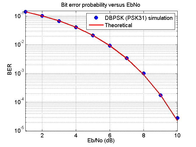
PSK31 is actually differentially encoded and should really be called DPSK31. Differential encoding is where the ones and zeros that make up the message are encoded as phase transitions rather than absolute phase values. This makes receiver design a lot easier and the receiver never experiences catastrophic loss of synchronization as can happen when not using differential encoding. However, if one bit goes wrong there’s a high probability that the next bit will also be wrong, this produces a greater BER for a given EbNo.
I am aware that there was no need to convert the baseband to the passband but I wanted to put the noise on the passband rather than the baseband for other reasons.
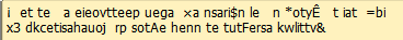
Running sound from Matlab via VB audio virtual cable to FLDIGI at 8 dB EbNo, FLDIGI decoded my message as “This is a¤SK31 test with AWGN added to the signal.”. At 6 dB I got “Thet iMa PSK31 eest with AW tN addef to the signal.”. So it looks like around 8 dB or a 99.9% probability of a successful bit transmission is needed for what I would consider reasonably acceptable communication but not perfect.
Reducing BER of PSK31 without increasing Eb/No or decreasing the net bit rate of PSK31
Other modulation schemes could be used but the only unencoded scheme I know that beats PSK31’s DBSPK modulation is BPSK and has an improvement of around 1 dB of Eb/No from what I can see but others say 2 dB. However, BPSK can be tricky to decode compared to DBPSK, therefore let’s stick with DBPSK.
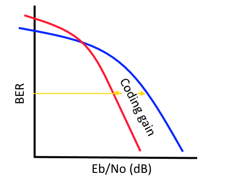
To reduce the bit error rate forward error correction (FEC) can be used. FEC means adding redundancy which means more data has to be sent which generally decreases net bit rate which I don’t want. However let’s first consider what happens, decreasing bit rate means bits take longer to be sent and hence Eb/No goes up but at the same time decreases BER. If BER goes down more than Eb/No goes up you can win for high enough Eb/No values and get a reduction in BER for a fixed Eb/No; this improvement is called coding gain. To measure the coding gain you have to specify a BER. To me it seems a BER around 10 − 5 (99.999% probability of a successful bit transmission) is an appropriate place to calculate coding gain and from what I’ve seen the seems to be a common place it is measured.
Trellis coded modulation (TCM) implements FEC without reducing net bit rate. It does this by increasing the constellation size so data can be sent quicker. For example, a BPSK is changed into a QPSK doubling the throughput meaning a 1/2 FEC convolution encoder can be used without affecting the net bit rate. The constellation and the convolution encoder in TCM are combined. So let’s see if we can make a differential TCM scheme for PSK31.
Matlab has no differential TCM but with a little bit of experimentation I think I have managed to clobber one together from a non-differential one. The figure below shows theoretical results for BPSK, DBPSK ( as used in PSK31) and DQPSK, in addition to my TCM-DQPSK.
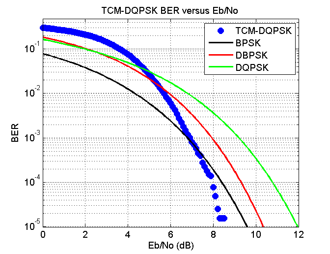
The net bit rate of TCM-DQPSK is identical to PSK31 but at a BER of 10 − 5 a gain of around 1 dB of EbNo can be obtained compared to DBPSK. TCM is easy to implement and I am surprised that no one has added this slight change to PSK31 for ham mode. The latency introduced with this modification to PSK31 would be 0.5 seconds for my implementation of it which would hardly be noticed. The bandwidth and the net bit rate would still be the same.
This simulation I added the AWGN to the baseband and never went into the passband and back down again as I did with PSK31.
Trying turbo codes
In Matlab I played around with turbo codes which is some sort of FEC that uses two convolutional coders in some sort of interleaving thing to produce codes that are apparently quite good. The best performance that seems to be obtained from them is to use soft decoding. Soft decoding is where you express the likelihood that a particular received symbol is say a one rather than saying it is definitely a one. This allows the decoder to weight paths accordingly. I was wanting a 1/2 rate encoder but the smallest one seems to be 1/3 ( one for the original data and to for both of the convolutional encoders ) therefore I had to puncture the code by removing every third element to obtain a 1/2 rate encoder. In Matlab you supply a block of data to a turbo encoder and it doesn’t seem to be able to be added bit by bit. The block of data has to align up exactly for the decoder to be able to decode it. This is a hassle as it requires some form of aligning the data correctly and the data is decoded block by block rather than a bit at a the time making the text output kind of jerky. Anyway, assuming the blocks have been aligned correctly I increased the constellation size to 4 and used DQPSK to send the encoded data; this way the net bit rate was again the same as PSK31. Simulating this I obtain the following figure.
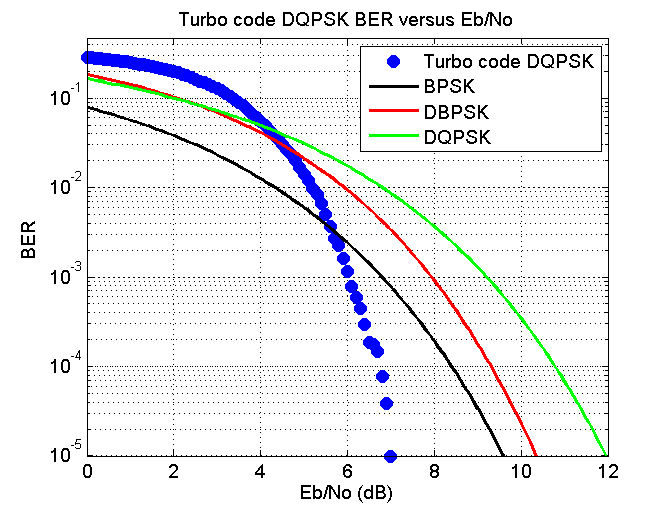
This time there appears to be a gain of around 2.5 dB
This simulation I added the AWGN to the baseband and never went into the passband and back down again as I did with PSK31.
LDPC
Low density parity check (LDPC) codes are some sort of FEC codes that are linear block codes. They have an interesting history of being invented in 1960 and more or less forgotten until 1996. Along with turbo codes they are currently hot topics in coding theory and applications. Like turbo codes they are apparently very good codes and seem to be battling it out as to who wins. Such codes are used for television like SVB-S2, DVB-T2, wifi like 802.11n and so forth (http://www.ldpc-decoder.com/en/ldpc-decoder-applications). A short introduction that I found useful can be found http://www.bernh.net/media/download/papers/ldpc.pdf. It seems the downside of LDPC codes is that they have to be reasonably long for them to be any good. From my mucking around with them on Matlab they are represented using a gigantic matrix mainly full of zeros, or what is called a sparse parity matrix. Matlab only comes with the DVB-S2 parity matrix and doesn’t give you any help on how to create other parity matrices for different applications. However, http://www.ldpc-decoder.com/en/ldpc-decoder-applications have a list of standards that use LDPC codes along with documentation that have a shorthand notation for such matrices. I obtained two different parity matrices 802.11n and one called G.9960, both are half rate encoders and have some of the shortest codewords I could find at 648 and 336 bits respectively. This means for PSK31 it would take approximately 10 seconds to send one G.9960 code or for QPSK at 31.25 bps 5 seconds. In Matlab the LDPC decoder has a soft decision-making process the same as I mentioned with turbo codes. Decoding of these codes uses something called belief propagation which is an iterative method and seems faster than whatever turbo codes use.
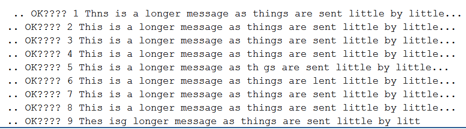
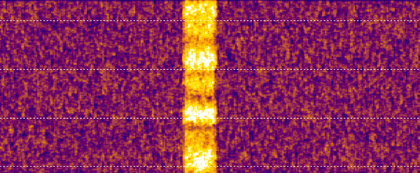
Like Matlab’s turbo codes LDPC codes are sent block by block making the text output jerky and the blocks have to align properly. Somehow the receiver has to align the bits it obtains after demodulation. I didn’t want to include any preamble so as to not include any overhead in the channel. To do this means the receiver has to find the codeword alignments unaided. For finding the alignment, when a bit came in, it was added to a buffer and soft decoding was done with only one or two iterations, the number of zeros in the parity check was then summed up. The idea was if the data received was aligned correctly then the received data would look more like a codeword than if it wasn’t meaning more zeros would be in the final parity check. Performing this every bit that came in, along with a peak search the following figure was obtained for the 802.11n using DBPSK at 31.25 bps with an Eb/No of 6 (very noisy conditions). For all experiments using LDPC I created the passband signal and added the AWGN to that before the standard symbol tracking and frequency tracking etc.
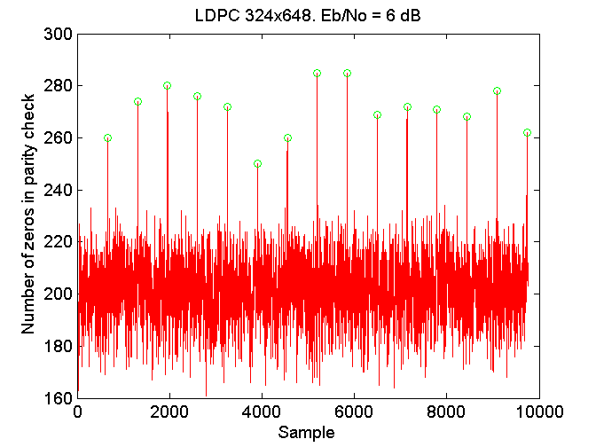
As can be seen there are clear peaks that represent the boundaries between codewords. I would imagine in the greater scheme this is an incredibly CPU intensive task but as the bit rate is so slow it’s laughable, a standard PC can do this without any problem at all.
Initially the program I wrote might obtain alignment but then an erroneous peak would appear that would unalign the code words again with disastrous results. A fix was to have a sort of reinforcement of a particular alignment which worked.
Setting an EbNo of 5.5 dB which is so noisy I could barely hear anything that sounded like a signal, and is way below the 10 dB EbNo required for normal PSK31 transmission, I ran my program with automatic alignment of codewords as just described and obtain the following picture.
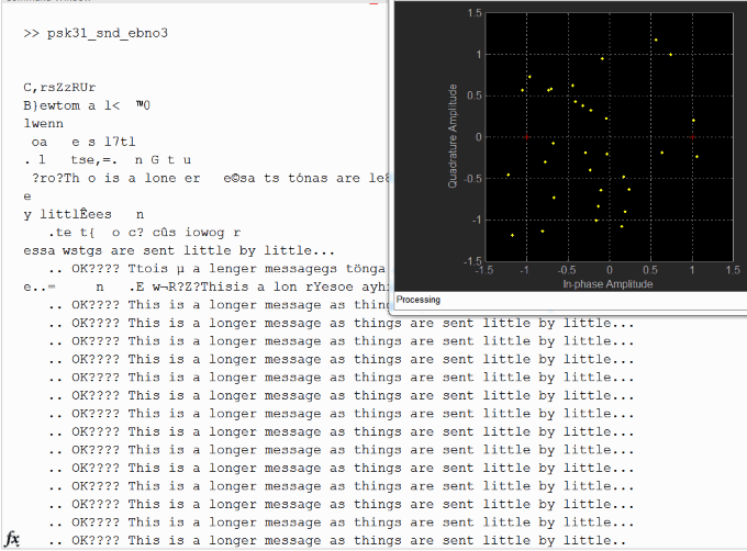
The first gobbledygook is mainly the thing trying to figure out the correct code alignment and symbol timing. There is no frequency offset in this test. You can see the received points do not look anything like what the constellation should be, but even still, it somehow manages to correctly decode every single codeword after that has correct alignment; this I find really really amazing. Of course as I was using BPSK the net bit rate was 15.625 bps (about 25 words per minute), which is a little slow I fear for most HAMs.
Switching over to DQPSK meant the speed went up to 31.25 net bps again (31.25 symbols a second). This time the AWGN was added to the passband for the BER versus EbNo plots. the following two figures show the results obtained from using the DVB-S2 and G.9960 LDPC codes.
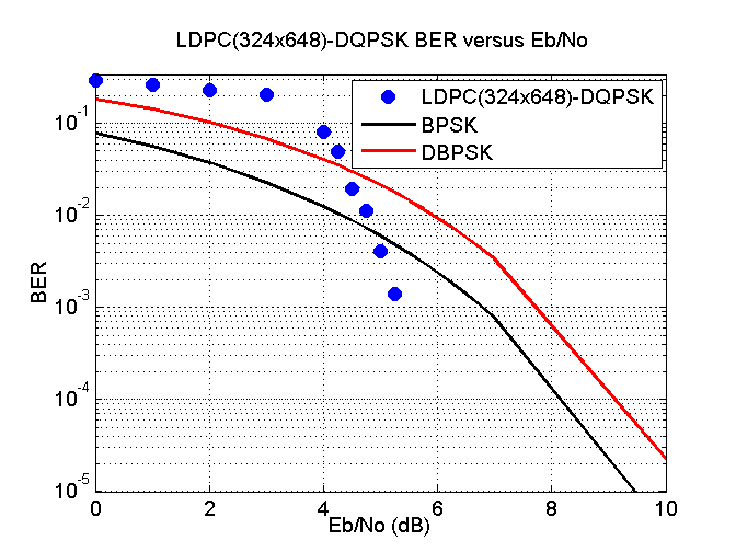
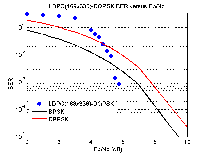
The net bit rate for both of these codes were 31.25 bits per second the same as PSK31 in addition to the same bandwidth as PSK31. The DVB-S2 was the best with the coding gain of around 4 dB but the code was slightly too long taking 10 seconds per code to be transmitted. G.9960 took about five seconds to transmit a codeword and had a coding gain of around 3.75 dB.
Meaningless SNR
Signal-to-noise ratio (SNR) seems to be quoted here there and everywhere. It’s even quoted on my soundcard as 114 dB, whatever that means. I definitely get confused when people quote SNR values as they always seem to differ so much. SNR is defined as “the ratio of signal power to the noise power” according to Wikipedia. The power of the signal is (1)/(RT)∑T − 1n = 0sig[n]2 and the power of the noise is (1)/(RT)∑T − 1n = 0noise[n]2. It gives you an idea of how loud a signal is compared to the noise. Dividing one formula by the other will not however likely give you an SNR value that matches anyone else’s. The main problem is with the noise and the fact that sampling limits the maximum frequency that can be represented, if you sample faster your noise will consist of more frequencies and as AWGN contains every frequency your calculation of the power of the noise will increase thus decreasing SNR. It makes no difference if you try to measure the power using some sort of analog device, as an analog device will have some bandwidth restriction which will also limit noise. The upshot is the power of the noise is technically infinite meaning SNR is always negative infinity in dBs.
To get around this problem people restrict the bandwidth before performing the calculation; this makes the power finite. However, generally no one mentions the bandwidth when quoting SNR and you have to guess which really grinds my gears. For oscilloscopes it may be 20 MHz, for a soundcard who knows, for HAM stuff it may be be 2.5 kHz, and for someone else it could even use the bandwidth of the signal to calculate the power of the noise over, who knows.
To make SNR more meaningful some notation like SNR2.5kHz, dB makes things clear as to what you’re doing. As HAMs on HF typically have receivers that have a bandpass of around 2.5 kHz when they make measurements of the noise this is the bandwidth they will be seeing hence my guess is that most SNR values seen on the Internet will be SNR2.5kHz when expressed by HAMs.
Personally I like C ⁄ N0 which normalizes the noise bandwidth to 1 Hz the same N0 noise density as we have seen before and C as the total signal power. This is normally written as CNo and I have commonly seen it used for satellite stuff (satellite TV and GPS). It has a nice interpretation that N0 = kBT where kB is the Boltzmann constant and T is temperature in Kelvin. CNo units are usually dB-Hz. CNo is a carrier to noise ratio (CNR). There seems to be a difference between carrier-to-noise ratio (CNR) and SNR depending where the measurement is performed but for me I’ll use them interchangeably and can’t promise that I’ll stick to one or the other. CNR apparently should be measured after transmission and before reception, while SNR should be measured before modulation or after demodulation in the baseband.
PSD and Power
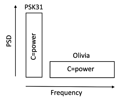
Power spectral density (PSD) is what people think as frequency displays; frequency along the bottom and PSD along the side.
The power of the signal is not the height of the PSD but rather the height times the bandwidth. The power of the two signals in the previous figure are the same despite the fact that the Olivia signal appears around 15 or 20 dB smaller on the PSD for any given frequency. You can’t just look at the height of the signal on a PSD and say a signal has that amount of power. Having some sort of needle that measures the total signal power coming in makes more sense than looking at a PSD display.
Meaningful SNR values
ki4SGU at http://ki4sgu.blogspot.co.nz/2009/11/signal-to-noise-ratio-raindows-in-dark.html seems like he had some way of measuring the μVs on his radio (probably some needle showing strength in μVs). I think he used this to determine SNR of various signals by 10log10⎛⎝(V2s)/(V2n)⎞⎠ where Vs was the voltage reading when the signal was present and Vn when the signal was not present. As his receiver I think would most likely have a bandwidth around 2.5 kHz the results he gives would be for SNR2.5kHz, dB. I too will follow this amount of bandwidth to calculate my noise over so I can compare my results with his. Below I quote what his findings were in what I believe is SNR2.5kHz, dB.
"CW@20WPM +3db (machine decoded by MFJ-461)
CW@20WPM +1db (machine decoded by fldigi or CWget)
HFpacket (300baud) +1db
RTTY45 -5db
CW@20WPM -7db (other claim like less, like -13db*)
PSK63 -7db
FELDHell -7db
PSK31 -10db
Olivia 64/2000 -13db
Olivia 16/500 -14db
WSPR -30db (maybe less)"
While a mode such as WSPR may be useful even when the CNo is much lower than PKS31, this does not in itself mean that WSPR is more energy efficient than PKS31 (i.e a lower EbNo for a given BER) it may be that WSPR spends way longer sending a bit than that of PSK31, so much so that even the small power that WSPR uses multiplied by time uses more energy per bit than PSK31 would use; however, it may not either.
SNR (CNR) EbNo relationship
In linear units and not in dB, the relationship between C and Eb is energy divided by time equals power which implies C = Ebfb where fb is the net bit rate. N and N0 is simply N = N0Bw. Therefore ...
SNRBw = (Ebfb)/(N0Bw)
If everything (bar fb and Bw) is in dB the formula becomes ...
SNRBw, dB = EbNodB + 10log10⎛⎝(fb)/(Bw)⎞⎠
So from Wikipedia, WSPR sends 50 bits of information taking 110.6 seconds meaning fb = 50 ⁄ 110.6 with a minimum SNR2.5kHz, dB = − 30dB obtained from ki4SGU we see that the energy efficiency of WSPR is EbNodB(WSPR) ≈ − 30 − ( − 37.4) = 7.4dB. Likewise we can do the same for PSK31 and obtain EbNodB(PSK31) ≈ − 10 − ( − 19) = 9dB. therefore, WSPR is actually more energy-efficient than PSK31, but I had no idea which was more energy-efficient until I did that calculation. As we have already seen, an EbNo of 9 dB has a BER of around 10 − 5 which is what I consider a low enough BER to be an good communication link.
For our LDPC-DQPSK modulation scheme at 31.25 symbols a second using the G.9960 LDPC code, from figure 8↑ we see that an EbNo of 6dB is around the minimum value for an acceptable communication link. Therefore...
SNR2.5kHz, dB(LDPC − DQPSK, G.9960) = 6 + ( − 19) = − 13dB
... which places our modulation scheme at Olivia 64/2000 according to ki4SGU. Our modulation scheme means the signal can still be successfully usable if the power of the transmitter is half compared to PSK31 while still maintaining the speed of PSK31.
There’s more to life than AWGN
So far we have only considered AWGN. AWGN is a channel impairment that is not particularly challenging. There are nastier channel impairments that happen in the real world. Of the nastier ones, ones with changing multipath environments and/or rapid Doppler changes are pretty nasty. As we seem to be dealing with a digital transmission scheme designed for HF it makes sense to simulate such HF channel impairments.
In Matlab you can model such HF channels with what it implements using the recommendations of ITU-R F.1487 for channel impairment modeling. Using it is as simple as the following for Medium latitudes, Moderate conditions (iturHFMM).
chan = stdchan(1/Fs, 1,’iturHFMM’);
chan.NormalizePathGains = 1;
chan.ResetBeforeFiltering=false;
sig_out = filter(chan, sig_in);
With Matlab high latitude conditions experience the worst conditions. For me living in the mid-latitudes when running voice through the filter the results sound uncannily like listening to a high power shortwave radio station.
So I’ll now stop adding AWGN and add just HF channel impairment without any noise added and see how the various modulation schemes perform.
HF channel impairments without AWGN
First putting PSK31 through HF, Medium latitudes, Moderate conditions (iturHFMM), and no AWGN, I obtain the following with my program which was almost identical mistake for mistake by Fldigi, and is shown in the following picture.
Using high latitudes moderate conditions (iturHFHM) instead both my program and Fldigi did not successfully decode anything of the original PSK31 message.
Similarly DQPSK at 31.25 symbols a second for iturHFMM was very successful and similar to that of DBPSK at 31.25 symbols a second, but when using iturHFHM it failed with DQPSK at 31.25 symbols a second. Trying all the HF channels that Matlab simulates I wrote down the following qualitative results that I got from them. From best to worst they are, excellent, good, marginal, terrible, total failure. They are only my personal opinion when trying to read the text that had been sent. It seems PSK31 is best for the mid-latitudes but does not do so well for either the low latitudes or high latitudes.
| Low latitudes | Medium latitudes | High latitudes | |
| Quiet conditions | good | excellent | good |
| Moderate conditions | marginal | good | total failure |
| Disturbed conditions | total failure | marginal | total failure |
| Disturbed conditions near vertical incidence | NA | terrible | NA |
Table 1 Qualitative PSK31 simulation results with no AWGN
Repeating the procedure again but using our new modulation scheme LCPC-DQPSK\strikeout off\uuline off\uwave off,G.9960 I obtained the following results where \uuline default\uwave default“excellent” means I did not see one error.
| Low latitudes | Medium latitudes | High latitudes | |
| Quiet conditions | excellent | excellent | excellent |
| Moderate conditions | excellent | excellent | total failure |
| Disturbed conditions | total failure | excellent | total failure |
| Disturbed conditions near vertical incidence | NA | excellent | NA |
Table 2 Qualitative LCPC-DQPSK\strikeout off\uuline off\uwave off,G.9960\uuline default\uwave default simulation results with no AWGN
You can see the ones that totally failed with PSK31 still fail with LCPC-DQPSK\strikeout off\uuline off\uwave off,G.9960. I read somewhere that these three total failures all have Doppler spreads of around 10 Hz which is an order of magnitude greater than any of the others. Anyway, interesting results.
HF, Medium latitudes, Disturbed conditions and AWGN
Adding AWGN back into the mix I compared DBPSK (PSK31) with LDPC(168x336)-DQPSK with varying amounts of noise to obtain the following bit error rate versus EbNo.
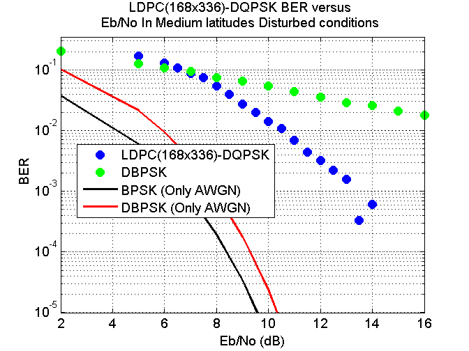
The results are quite shocking. For LDPC(168x336)-DQPSK there is a slow decrease of BER between 6 dB and 13 dB rather than the sharp cliff looking response as can be seen in figure 8↑. After around 13 dB there is a better decrease in BER and above 15 dB I did not detect any errors with LDPC(168x336)-DQPSK. So in the presence of Medium latitudes Disturbed conditions there is approximately a 9 dB cost involved. This means you would need a transmitter eight times more powerful due to the presence of Medium latitudes Disturbed conditions compared to if there was just AWGN to deal with. Still, it’s a lot better than DBPSK (PSK31) where errors were detected no matter how much power your transmitter has.
Finally putting a single tone through the channel rather than modulating it I looked at what the channel does to what amounts to being a continuous stream of repeating constellation points, this you can see in the following figure.
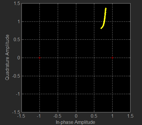
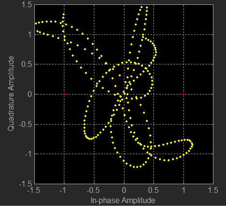
I tried high and mid latitudes under moderate conditions. for the mid-latitudes the pilot did not move particularly fast, and it was easy to tell visually where the offset was. For the high latitudes the thing just went nuts and would move extremely fast; it moved too fast to visually predict where it would be fraction of a second later. So we could send data quicker and use more bandwidth so that we see the pilot move less due to the Doppler between one symbol on the next; let’s try that.
62.5 symbols a second
Using LDPC(336x672)-DQPSK and 62.5 symbols a second means the points on the IQ display can only move half the speed that they used to due to Doppler. Trying this I got the marginal quality link (about 2% error) on moderate conditions high latitude which can be seen from table 2↑ I couldn’t at 31.25 symbols a second. This trick also worked at 125 symbols a second but not at 250.
Also with LDPC(336x672)-DBPSK at 62.5 symbols a second I was able to get a marginal link quality on disturbed conditions at low latitudes. That leaves just disturbed conditions at high latitudes.
Matlab Code
I put together a modem written in Matlab to demonstrate my LDPC-DQPSK31 protocol which you can obtain here ldpc-dqpsk31-modem.zip
It modulates and demodulates in the passband that can be sent out to the soundcard and obtained from the soundcard. I wrote it in MATLAB R2014a and it requires the comms and dsp toolboxes. Just type LDPC_DQPSK31 into the command window and the program will run with a constellation display and you will hear the sound as well as it will decode the sound. I am aware that the frequency tracking of it is probably not particularly great and should be changed but as I wasn’t testing how well it could cope with frequency drift I wasn’t too concerned with this.
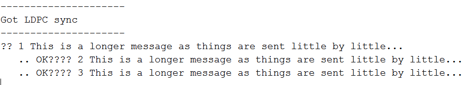
For those who don’t have Matlab here is some sound the program produced ldpc-dqpsk31.wma and below is what the program outputted on the command window.
Others might find the files varicode_init.m varicode.txt vari_encode.m vari_decode.m useful for making a PSK31 modem. These files will encode and decode PSK31 varicode.
Jonti 2015
Home
Home